Study notes
Regression
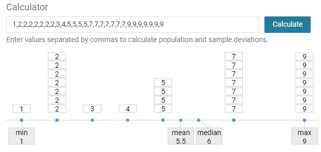
mean
The average value of the given observations
median
The middle value of the given observations.
If there are two values in the middle, then median is a dataset.
1,2,3,4,5,5,5,5
1,2,3 5,5,5
4,5 (four and five)
In computation is taken the average between values.
mode
The value that appears most often in a set of data.
It is the value that is most likely to be sampled.
Value seen most often
If more than one value is seen the same times, then mode is a dataset contain all these values.
 In computation is taken the first one (most common)
range
the area of variation between upper and lower limits on of the given observations
max value - min value
Explained variance
Variance in the response variable (label) in a model that can be explained by the predictor variable(s) (features) in the model.
Between 0and 1
The higher the explained variance of a model, the more the model is able to explain the variation in the data
Explained variance appears in the output of two different statistical models:
2. Regression: Used to quantify the relationship between one or more predictor variables and a response variable.
Variance
It is calculated by taking the average of squared deviations from the mean. Variance tells you the degree of spread in your data set.
((y1-mean)2 +.... (yn-mean)2/N
Z-Score
Measurement that describes a value relationship to the mean of a group of values
Technically, it measures the standard deviations below or above the mean. It ranges from -3 standard deviation up to +3 standard deviation.
Help to understand how far the data point is from the mean.
standard deviation (STD)
Measure of how dispersed the data is in relation to the mean.
The most useful. It provides a measure of variance in the data on the same scale as the data itself.
Low standard deviation means data are clustered around the mean, andhigh standard deviationindicates data aremore spread out.
Relative Squared Error (RSE)
A relative metric between 0 and 1
It is based on the square of the differences between predicted and true values.
The closer to 0 this metric is, the better the model is performing.
It can be used to compare models where the labels are in different units.
Relative Absolute Error (RAE)
A relative metric between 0 and 1
It is based on the absolute differences between predicted and true values.
The closer to 0 this metric is, the better the model is performing.
It can be used to compare models where the labels are in different units.
Mean Absolute Error (MAE)
The average difference between predicted values and true values.
This value is based on the same units as the label, in this case dollars.
The lower this value is, the better the model is predicting.
#y = actual value
#y^ = predicted value
((y1-y1^) + …… (yn-yn^))/N
#y^ = predicted value
((y1-y1^) + …… (yn-yn^))/N
Mean Square Error (MSE)
The mean of the squared differences between predicted(y) and actual values(y^).
This is a relative metric, which the smaller the value, the better the fit of the model
# y = actual value
# y^ = predicted value
((y1-y1^)2 + ... (yn-yn^)2)/N
# y^ = predicted value
((y1-y1^)2 + ... (yn-yn^)2)/N
Median Absolute Percentage Error (MDAPE)
It is the median of all absolute percentage errors calculated between the predictions and their corresponding actual values.
Median absolute error
Should be like above but refer to median of all errors calculated between the predictions and their corresponding actual values.
Normalized mean absolute error
Normalized median absolute error
Normalized root mean squared error
Normalized root mean squared log error
Root mean squared log error
Spearman correlation
To Be
Normalized median absolute error
Normalized root mean squared error
Normalized root mean squared log error
Root mean squared log error
Spearman correlation
To Be
Root Mean Square Error (RMSE)
The square root of the MSE.
Result an absolute metric in the same unit as the label.
The smaller the value, the better the model (in a simplistic sense, it represents the average number of rentals by which the predictions are wrong!)
Root square of MSE
residuals
The difference between the predicted and actual value (evaluate Regression trained model)
Indicates the amount of error in the model.
# y = actual value
# y^ = predicted value
y-y^
# y^ = predicted value
y-y^
RSS
sum of squares of residuals
# y = actual value
# y^ = predicted value
(y1-y1^)2 + ... (yn-yn^)2
TSS
How much variation there is in the observed data (total residuals)
# y = actual value
# y^ = predicted value
(y1-y1^) + ... (yn-yn^)
Coefficient of Determination (R-squaredor R2)
How much of the variance between predicted and actual label values the model is able to explain.
A relative metric in which the higher the value, the better the fit of the model.R2 = 1-RSS / TSS
Classification
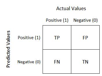
True negative (TN)
Value predicted is 0, the actual value is 0
True positives (TP)
Value predicted is 1, the actual value is 1
False negatives (FN)
Value predicted is 0, the actual value is 1
False positives (FP)
Value predicted is 1, the actual value is0
Confusion Matrix
Summary of prediction results on a classification problem
Binary classification
 sklearn.metrics.classification_report
return the confusion matrix like this:
Predicted - X
Actual - Y
TN | FP |
FN | TP |
Accuracy
Out of all prediction how many the model identified correct.
(TP+TN) / (TP+FP+TN+FN)
Recall
True Positive rate out of all actual Positive
Out of all Identified positive how many were identified correct (actual positive were identified positive)
Out of all of the values in dataset, what proprtion the model has identified correct.
TP/(TP+FN)
Precision
Out of all predicted Positive how many were Positive (predicted Positive were identified correct)
Of the predictions the model made for this class, what proportion were correct
TP/(TP+FP)
False positive rate
Opposite of Recall (True positive rate)
Out of all Identified positive how many negative were identified correct (actual negative were identified negative)
Number of negative cases incorrectly identified as positive compared the number of actual negative cases
FP/(TP+FN)
F1-Score
The average (harmonic mean) of precision and recall.
(Recall + Precision) / 2
Micro average
The function to compute f1 by considering total true positives, false negatives and false positives (no matter of the prediction for each label in the dataset)
Macro average
The function to compute f1 for each label, and returns the average without considering the proportion for each label in the dataset.
Returned in classification_report()
Weighted average
The function to compute f1 for each label, and returns the average considering the proportion for each label in the dataset.
Returned in classification_report()
Sample average
The function to compute f1 for each instance, and returns the average.
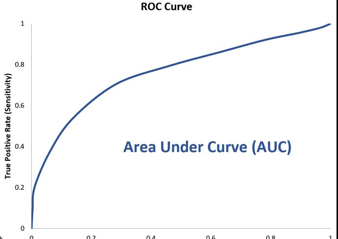
ROC curve (curve)
Receive Operatic Characteristic
The curve of the True Positive (TP) and False Positive (FP) rates for different threshold values between 0 and 1
Y axis -True Positive Rate (Recall)
X axis - False Positive rate
sklearn.metrics.roc_curve
Return:
fp- rndarray of shape (>2,) - False Positive Rate
Increasing false positive rates such that element i is the false positive rate of predictions with score >= thresholds[i].
tpr- ndarray of shape (>2,) - True Positive RateIncreasing true positive rates such that element i is the true positive rate of predictions with score >= thresholds[i].
thresholds - ndarray of shape = (n_thresholds,)- Decreasing thresholds on the decision function used to compute fpr and tpr. thresholds[0] represents no instances being predicted and is arbitrarily set to max(y_score) + 1.
We have:
x_test
array([0, 0, 1, ..., 1, 1, 1], dtype=int64)
y_score= model.predic_proba(X_test)[[0.81651727 0.18348273]
...
[0.63865894 0.36134106]]
# Runfpr, tpr, thresholds = roc_curve(y_test, y_scores[:,1])
Thresholds: [1.9971475 0.9971475 0.9890549 ... 0.0284842 0.02845313 0.00998016]
AUC
Area Under the Curve
Value between 0 and 1 that quantifies the overall performance of the model. The closer to 1 this value is, the better the model
Support
Score evaluation in multi class classification.
Show how many instances of this class are there in the test datasets
Imbalanced support in the training data may indicate structural weaknesses in the reported scores of the classifier and could indicate the need for stratified sampling or rebalancing.
predict_proba
In classification return the probability of a label.
Clustering
Average Distance to Other Center
How close, on average, each point in the cluster is to the centroids of all other clusters.
Average Distance to Cluster Center
how close, on average, each point in the cluster is to thecentroid of the cluster.
Number of Points
The number of points assigned to the cluster.
Maximal Distance to Cluster Center
The maximum of the distances between each point and the centroid of that point’s cluster. If this number is high, the cluster may be widely dispersed.
Cluster’s spread
Statistics
Maximal Distance to Cluster Center AND Average Distance to Cluster Center
References:
User guide: contents — scikit-learn 1.2.1 documentation