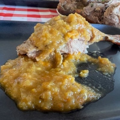
Duck a l'Orange

French recipe
Duck à l'orange as a tired cliché of the 1960s,


  • Active Time: 45 min
  • Total Time: 2 1/4 hr
  • Makes 4 servings

Ingredients:
For duck
1 tablespoon kosher salt
1 teaspoon ground coriander
½ teaspoon ground cumin
1 teaspoon black pepper
1 (5- to 6-lb) Long Island duck (also called Pekin)
1 juice orange, halved
4 fresh thyme sprigs
4 fresh marjoram sprigs
2 fresh flat-leaf parsley sprigs
1 small onion, cut into 8 wedges
½ cup dry white wine
½ cup duck stock, duck and veal stock*, chicken stock, or reduced-sodium chicken broth
½ carrot
½ celery rib
For sauce
⅓ cup sugar
⅓ cup fresh orange juice (from 1 to 2 oranges)
2 tablespoons white-wine vinegar
⅛ teaspoon salt
2 to 4 tablespoons duck or chicken stock or reduced-sodium chicken broth
1 tablespoon unsalted butter, softened
1 tablespoon all-purpose flour
1 tablespoon fine julienne of fresh orange zest, removed with a vegetable peeler
Special Equipment
an instant-read thermometer; a 13- by 9-inch flameproof roasting pan

Method:
Roast duck:
Step 1
Put oven rack in middle position and preheat oven to 475°F.

Step 2
Stir together salt, coriander, cumin, and pepper. Pat duck dry and sprinkle inside and out with spice mixture. Cut 1 half of orange into quarters and put in duck cavity with thyme, marjoram, parsley, and 4 onion wedges.

Step 3
Squeeze juice from remaining half of orange and stir together with wine and stock. Set aside.

Step 4
Spread remaining 4 onion wedges in roasting pan with carrot and celery, then place duck on top of vegetables and roast 30 minutes.

Step 5
Pour wine mixture into roasting pan and reduce oven temperature to 350°F. Continue to roast duck until thermometer inserted into a thigh (close to but not touching bone) registers 170°F, 1 to 1¼ hours more. Turn on broiler and broil duck 3 to 4 inches from heat until top is golden brown, about 3 minutes.

Step 6
Tilt duck to drain juices from cavity into pan and transfer duck to a cutting board, reserving juices in pan. Let duck stand 15 minutes.

Make sauce:
Step 7
While duck roasts, cook sugar in a dry 1-quart heavy saucepan over moderate heat, undisturbed, until it begins to melt. Continue to cook, stirring occasionally with a fork, until sugar melts into a deep golden caramel. Add orange juice, vinegar, and salt (use caution; mixture will bubble and steam vigorously) and simmer over low heat, stirring occasionally, until caramel is dissolved. Remove syrup from heat.

Step 8
Discard vegetables from roasting pan and pour pan juices through a fine-mesh sieve into a 1-quart glass measure or bowl, then skim off and discard fat. Add enough stock to pan juices to total 1 cup liquid.

Step 9
Stir together butter and flour to form a beurre manié. Bring pan juices to a simmer in a 1- to 2-quart heavy saucepan, then add beurre manié, whisking constantly to prevent lumps. Add orange syrup and zest and simmer, whisking occasionally, until sauce is thickened slightly and zest is tender, about 5 minutes. Serve with duck.


References: https://www.epicurious.com/recipes/food/views/duck-a-lorange-233535


Pasta con Melanzane e Pesce Spada - Pasta with Eggplant and Swordfish

Find your soulmate

We, as human being, are social individuals. We feel fulfilled as a person in our society when we have people around us. The right person at your side can double your happiness. We carry within us the desire to communicate, to exchange ideas and feelings. Our life is structured around communication and belonging to a family, a family which offer us membership, protection and offspring.
Isolated persons are prone to mental illness.

What is love?

Love is the feeling that your partner completes your life as a family. Man and woman fall in love because they are two parts of one whole (from society perspective). Man is aggressive and protective, woman is nurturing and demure. So, they complete each other. (NB: each person (woman or man) is complete by him/her self and nobody will interfere with that person inner value. Each person is unique and valuable throughout our humanity).
Love for woman is different from the love for man. For woman perspective the love is beautiful and complete: everything about her lover is perfect and beautiful and a flow of emotional feelings are exploding. Her love will lead her to having sex. For man, love is frustration. He is driven by sexual desires. He love the sexual parts of woman body: the legs, the breasts, the bottom... As for woman love represents empathy (she is there for her man needs: from carrying for her man to showing him affection and consideration), for man love is action (he dominate his woman, protect her and spread his sperm). This is way after sex, woman is loving and in need for caresses, while man is willing to rest and restore his energy to be ready for next action.
However, when a man love the face of his partner, he loves his mother memory.

Is love about looks? You may say so. If a good looking person is appealing to you is because that person look represents the guarantee that he / she is a healthy person with a good chance to produce offspring. Those are the persons with sex appeal and are generally accepted as good looking.
In same category with looks can be included hormonal chemistry between sexual partners. Through hormones are transmitted messages of being sexual potent and available for the person in front of you.
But beauty can incorporate other body characteristic, beside the classical ones. For example that person reminds you about a parental figure, a figure that produce you the familiarity feelings, closeness and offers you comfort and protection. The subject is detailed in the section "How we choose our partner?".
Looks and sexual attraction are not everything in a relationship. Sexual attraction can vanish in time (it is a novelty driven instinct), love is something which should grow in time and consolidate your family through attachment ( it is comfort, security, provides you a pleasant life and happiness). So, another manifestation of love is mental affinity. If the couple has same set of values in life and likes same activities, they can build a future together. (see
Happiness and rational thinking - Pleasant life and Life with meaning).
Admiration is another component of love. When we admire a person, we cherish his / her companionship.
And finally, we are talking about emotional affinity. Feelings are the cause of falling in love.

In our society it is generally accepted that if you love someone, you commit to monogamist relationship with that one. And if you have an affair, it means that you are not in love with your partner anymore. Monogamy is simply an agreement: Woman trades sexual fidelity to man in exchange for protection and his commitment to provide for her and her offspring. Monogamy is a society rule and represents the insurance that the man will spend his life beside his woman and his biological children, he will not provide for other men's children, exception if he adopt existing woman's children. Exceptions are only to enforce the rule.

How to look for him / her when choosing the right person?

First of all, you need to be open for a new relationship. No matter how were your past experiences, everyone can have a good life with the one. You have to be optimist: to want to find the right person, to believe that does exist a soulmate for you and that you can find it.
Mental set is always a must: to experience love, you need to believe in it. Self-esteem is also important: believe that you are worth loving and that you are able to find the right person to love and be loved.
With positive attitude, start a new relationship with sincerity and communication (lack of communication is one of the causes which make a relationship to fail) and give what you want to receive from this relationship (behave with your loved one the way you want her / him to behave with you, be open to your feeling in your relationship).

Learning how to menage your life in two, is not the easiest thing to do: you will see and you will be expose in all kinds of situations pleasant or less pleasant. You need to develop your acceptance: The degree of cleanliness accepted in the couple must be that of the cleanest of them. The degree of humility accepted in the couple must be taken into account by the humblest of them. If these limits are exceeded, frustrations and tensions will be created in the couple and can even lead to the breakup of the couple.
Spend as much time together as possible. Engage both of them in daily activities.
Spend time together doing what you both like to do (hobbies).
Try new activities which appeal to one of you, the other may love it.

Look for similar hobbies and wishes in your life. These will make your life together easy to menage (see Happiness and rational thinking - Pleasant life).

Choose a partner with similar background: social, cultural and economic. If you share similar values, your love will be able to last (see Happiness and rational thinking - Life with meaning).

Choose a partner with similar sexual expectation. Sex is part of your couple life and can create frustration in time (sex as bounding not only procreation). If you wish children, make sure that your partner feels the same way.

Choose the partner who can provide you the life you dream of. If you, as woman, wish a luxuriant life, you should choose a partner financial potent. If you, as men, wish to have home made meals, you should choose a partner with cooking abilities. If you are a party person, you should make sure your partner likes to party as well. And so on...

Choose a partner to be proud of. Admiration is a big thing in relationship. Choose a partner with defects which are not capital for you. It may not be altogether only qualities, but at least you to be able to accept the defects and learn to diminish them into your eyes. Learn to love your partner with good and bad.

It is said that woman is making the decision of getting together into a relationship. Naturally, she will choose a partner financial potent (but not only) to ensure her material well-being for her and her eventual children.

Harmful behaviors in the couple's relationship

Adoration is a behavior which creates rejection because of sick reactions such as abandonment issues.

Psychic anaphrodisiacs (sexual inhibitors):
For men: Thinking of their mother (the most asexual presence in the life of a sexually mature man). Keep away from relationship with a woman which resembles your mother face.
Another powerful psychic anaphrodisiac for men is the presence of another man from the life of his partner (talking about too many details in regards with the performances of the other man in the past of his partner). As woman: keep for yourself the details of your past relationships.
For woman: all the unsafely situations, especially those regarding the future of the relationship will act as psychic anaphrodisiac.

A little routine helps us build a good, strong relationship; but take it too far and it destroys and “kills love.” Finding the balance is up to you.

Confusing behaviors in the couple's relationship

Invariable erotic behavior is manifested through contradictions between verbal and non-verbal language: he/she likes it, then he/she doesn't like it anymore.
Young people may manifest indifference to the person attracted due to the instinct of egos specific to children combined with irresistible attraction to a possible partner.

Beneficial behaviors in the couple's relationship

Jealousy feeling for men is good to cancel the effects of selfishness.

The woman appreciates the compliments related to her beauty, while the man appreciates the compliments related to his deeds.

The place of intimacy between two partners is very important for the woman (she remembers):
- it must be clean and have a bathroom,
- it must provide safety
- and the ambience matters a lot.

To be good in bed means:
- movements that produce a complex of multisensory perceptions (smell (pheromones), skin color, clothes),
- confidence
- and curiosity, spontaneity, the desire to get to know your partner.
If you feel good, you can help your partner to feel good as well. It is a circle. As a woman, you should tell to your partner that he is good in bed.

The expectation theory: Before an event, people are making a "projection" of what will happen. Going on a date, the woman expects something romantic, and the man expects to have sex. It is a conflict situation between the two partners: on the one hand, there is a conflict between her and his expectations, on the other hand, there is a conflict between everyone's expectations and what will happen for real. This conflict situation leads to disappointment.
Men make exaggerated promises to get what they want (the theory of expectations). As men, if you want a harmonious relationship, promise only what will be fulfilled and thus you will enchant the chosen one of your heart.

How we choose our partner?

We have our subconscious formed in our firsts years. In this way, our life is programed in proportion of 95% before we start dating. It is written in our subconscious through our experience at the moment of our childhood.
How we like someone based on our subconscious? We choose to like someone who is familiar to us, maybe someone who reminds us of a parental figure. The person who show us love, who cared for us. That person can be good or bad for us as per the childhood's experiences. So, the life trap is that we might end up in a toxic relationship because of the experiences written in our subconscious. Somebody from our family may caused us traumas which we learn to live with and we are choosing the person who cause us similar traumas in present. This kind of life we know to deal with, it is familiar to us, the lack of trauma is the unknown.
The unknown (good or bad) is what we reject. The familiar, good or bad, we accept because we have a previsions experience, we know how to face it.

When I know I am in a toxic relationship and I need to separate?

Toxic relationship is the one which it creates great and recurrent discomfort to one of the partners in relationship:
- physical or mental or emotional abuse (include traumatic jealousy)
- not having and maintaining same propose in life (include the decision to have children) (see Happiness and rational thinking - Life with meaning).
- promiscuous behavior of one or both partners (adultery)
The first thing in finding a solution for a toxic relationship is to realize that you have a problem and to take decision about it. You may need professional help.

Marriage:

Marriage is the promise and commitment to have a monogamist relationship for the rest of your life. Not all marriages are "for ever", but this "for ever" is the initial intention.
Marriage is usually more appealing to women than to men, because women are driven to have a family (to get the protection and the care from a man) and to have children. The necessity of given birth is in her genes. Almost every woman carries in her mind the idea to became mother in a certain point of her life. Little girls are playing the motherhood role with their dolls and this role will became a directive of her subconscious. The reproductive instinct is very strong and the man should take it into account when propose a woman to marry him.
When men initiate the marriage is often more about commodity of sex than the reproductive instinct. This does not mean that men never want children in their life, but they will delay the moment of being responsible for their kids and to have all the wives attention for themselves. For men, having kids is not always the propose of the marriage.

So, what about having children? There are situations when partners have two different propose of their marriage. One to have children and the other to get sexual commodity. When this is the case, the couple has a big problem. The true way to solve this problem is the divorce: if a child was born during the marriage, mother take the child custody while the father is contributing financial to his child care. If there is no child involved, the woman have to find the right man to start a family with, family which includes children.

It is another situation when marriage occurs: two people which wish to avoid loneliness, to double the fun and happiness in their lives or to find help in each other in difficult moments of life. Usually, it is the case of the late marriage.


NEW ENTRIES

DIY Dry Cleaning Solvent

No category

French cuisine

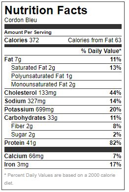
CORDON BLEU


This dish is originally from Switzerland, although today it is widely spread throughout France.


Cordon bleu is a cutlet of veal, pork, chicken or turkey rolled around ham and cheese, breaded and then cooked.

Prep Time: 20minutes mins
Cook Time: 30minutes mins
Resting Time: 45minutes mins
Total Time: 50minutes mins
Course: Main Course
Cuisine: French, Swiss
Servings: 2 people

Ingredients:
  • 2 veal cutlets (or pork or chicken cutlets)
  • 1 large slice raw ham
  • 150 g Comté cheese
  • 1 large egg
  • 4 tablespoons all-purpose flour
  • 6 tablespoons breadcrumbs
  • Salt
  • Pepper
  • Butter (or clarified butter or sunflower oil, for cooking)

Method:
  1. Butterfly the cutlets.
  2. Depending on their size, flatten them a little using a meat mallet. Lightly season with salt and pepper.
  3. Cut the slice of ham in half.
  4. On each flattened cutlet, place a piece of ham, then thin slices of Comté.
  5. Fold each cutlet in half and place in the refrigerator for 45 minutes.
  6. Pour the flour into a deep dish.
  7. Beat the egg in a second hollow dish.
  8. Pour the breadcrumbs into a third hollow dish.
  9. Roll the first cordon bleu in the flour and tap it to remove the excess.
  10. Then dip it in the egg.
  11. Finally, roll it generously in the breadcrumbs.
  12. Proceed in the same way for the second cordon bleu.
  13. Preheat the oven to 300 F (150°C).
  14. Heat a generous amount of fat (butter, clarified butter or sunflower oil) in a skillet over medium heat.
  15. As soon as the fat reaches a temperature of 340 F (170°C), dip each cordon bleu into it and fry them on both sides, until golden brown.
  16. Remove the cordons bleus, place them in a baking dish, and bake for 10 to 15 minutes.


This dish is commonly served with French fries, mashed potatoes, rice or even salad.

VARIATIONS
Throughout the world, the versions of different types of meat breaded and then fried are countless – and there are also many that include cheese inside. Traditional cordon bleu can be prepared with a few variations, including baking instead of frying, placing ham on top of the chicken, using bacon instead of ham, or eliminating the breadcrumb coating altogether.

There is even a version called “cordon bleu de prosciutto” which is ham wrapped around cheese and mushrooms.

In Spain, specifically in the province of Asturias, there is cachopo. This dish is nothing more than a beef or chicken cutlet rolled up just like cordon bleu and stuffed with Serrano ham and some melting cheese. Generally, if it is the version made with chicken, it is called San Jacobo.

Finally, in Uruguay and Argentina, people use the term “stuffed milanesa“. The milanesa is nothing more than a filet of beef, pork, chicken or fish in batter and fried, and in its stuffed version, it is simply folded in half and stuffed with ham and mozzarella cheese.


Reference:
See on Authentic French Dishes
https://www.196flavors.com/cordon-bleu/

DAUBE


Daube comes from the South of France and is one of the most famous of Provencal stews.

The word “daube” comes from the Provençal word adobar which means “to prepare or arrange”. The genius of the cooks who invented this stew was to prepare a tasty dish with ingredients of mediocre quality. “Adobo” in Provençal would mean “to arrange”, therefore to “improve”.


Daube is a traditional comforting French stew from Provence made with beef that is marinated in red wine with herbs and spices.
Prep Time: 30minutes mins
Cook Time: 6hours hrs
Rest Time: 8hours hrs
Total Time: 6hours hrs 30minutes mins
Course: Main Course
Cuisine: French
Servings: 6 people


Ingredients:
For the marinade:
  • 1 kg beef flank (cheek, chuck or beef stew)
  • 1 carrot , cut into 1-inch/2,5cm sections
  • 1 onion
  • 4 cloves garlic
  • 1 bottle Provence red wine (preferably full-bodied)
  • 3 cloves
  • 1 leek (white part), cut into 3
  • 1 stalk celery
  • 1 bouquet garni (thyme, rosemary, savory, and laurel)
  • 3 strips orange zest
  • Salt
  • Pepper
For the stew:
  • 4 carrots , cut into 2-inch/5cm sections
  • 3 shallots , finely chopped
  • 1 onion , finely chopped
  • 1 slice smoked pork belly , diced
  • 1 cup black olives , pitted
  • 2 tomatoes , peeled, seeded, and coarsely chopped
  • 1 tablespoon flour
  • 6 tablespoons olive oil
  • Salt
  • Ground pepper

Method:
Marinade:
  1. The evening before, cut the beef into large chunks and place in a large bowl.
  2. Add the onion, cut into 4, and with the cloves inserted. Add the carrot, 2 garlic cloves lightly crushed with the flat side of a knife and 2 pressed garlic cloves. Add bouquet garni and orange peels. Season with salt and pepper. Cover with red wine. Mix well.
  3. Cover with plastic wrap and let stand for at least 8 hours in the refrigerator. Mix the marinade two or three times during this time.
Stew:
  1. Drain the pieces of meat with a skimmer and place on paper towels. Reserve the marinade.
  2. In a cast iron pot, Dutch oven or an electric slow cooker, heat the olive oil and sweat the shallots and onion over medium heat.
  3. Add the smoked pork belly, and sauté for 3 minutes over medium heat. Add the meat, and brown the pieces of beef on each side.
  4. Pour the flour gradually and stir with a wooden spoon.
  5. Add the tomatoes, season with salt and pepper and mix again.
  6. Remove the celery and leek from the marinade and add the marinade to the pot. Cook 1 minute over high heat and simmer over very low heat for 5 to 7 hours or more.
  7. Two hours before the end of cooking, add the carrots and black olives. Ensure that the sauce does not completely evaporate during cooking.

Notes
Hock, round, flank, cheek, ox tail, scoter and neck are also the different beef cuts that can be used for this recipe.
You can use a pressure cooker to reduce the cooking time but it will be necessary to regularly monitor the level and the smoothness of the sauce.
Serve with steamed potatoes, mashed potatoes, or pasta.

Reference:
https://www.196flavors.com/france-daube/

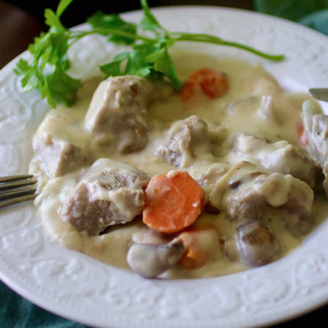
BLANQUETTE DE VEAU


Blanquette de veau (veal blanquette) is a veal stew that is definitely part of the French culinary heritage.
Some historians believe that the blanquette would be the evolution of a classic recipe of the Middle Ages called brouet de poulet.
Other versions attribute the paternity of blanquette to Vincent La Chapelle (1690-1746), a French cook who was the chef of Lord Chesterfield in England and then of the Prince of Orange-Nassau, before becoming the chef of Madame de Pompadour and finally Louis XV.


Blanquette de veau is a traditional French dish known for its delicious creamy white sauce prepared with creme fraiche and egg yolks.

Prep Time: 30minutes mins
Cook Time: 1hour hr 30minutes mins
Total Time: 2hours hrs
Course: Main Course
Cuisine: French
Servings: 4 people


Ingredients:
  • 1 kg veal , shoulder, chest or flank, cut into large cubes
  • 1 onion , poked with whole cloves
  • 1 bouquet garni (parsley, thyme, bay leaf, sage)
  • 4 carrots , cut into large sections
  • 250 ml dry white wine
  • 300 g mushrooms , quartered
  • 50 g butter
  • 50 g flour
  • 200 ml creme fraiche
  • ½ lemon , juiced
  • 3 egg yolks
Method:
  1. Put the meat cubes in a large saucepan and cover with cold water. Bring to a boil and add salt.
  2. Skim regularly at the surface so that the broth becomes clear. After 20 minutes, add the onion stuck with cloves and the bouquet garni.
  3. Simmer for another 20 minutes, then add carrots and wine.
  4. Continue to simmer uncovered over low heat for another 45 minutes or until meat is tender. Add a little water during cooking if necessary. Remove the onion and the bouquet garni.
  5. Meanwhile, sauté the mushrooms in a frying pan for 2 minutes with a knob of butter. Add salt, pepper, add a ladle of broth and continue cooking for 5 minutes.
  6. Sauce (prepare a few minutes before serving)
  7. In a saucepan, melt the butter. Add the flour while whisking over low heat for 5 minutes.
  8. Gradually add cooking broth while whisking until a reaching a thick sauce consistency.
  9. Add creme fraiche as well as lemon juice, and continue cooking for 2 minutes.
  10. Take saucepan off the heat and add egg yolks. Whisk well to incorporate. Add this sauce back to the pan with the meat and vegetables. Add the mushrooms and gently stir to incorporate everything.
  11. Immediately serve the blanquette with rice.

Reference:
https://www.196flavors.com/france-blanquette-de-veau/

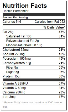
HACHIS PARMENTIER

Hachis parmentier is a popular family dish named after the apothecary and pharmacist Antoine Augustin Parmentier. The latter was an avant-garde scientist who lived in the 18th century.


Hachis Parmentier is a French dish made from mashed potatoes and shredded, finely minced or ground beef.
Prep Time: 30minutes mins
Cook Time: 1hour hr
Total Time: 1hour hr 30minutes mins
Course: Main Course
Cuisine: French
Servings: 4 people
Calories: 546kcal


Ingredients:
  • 6 potatoes , about 3 lb / 1.2 kg
  • 400 g shredded or knife-chopped beef , ideally leftover stew meat
  • 1 carrot , finely diced
  • 1 onion , grated
  • 2 cloves garlic , pressed
  • 2 tablespoons olive oil
  • 1 tablespoon thyme
  • 120 ml heavy cream
  • 120 g grated cheese (Gruyère, Emmental or Comté)
  • Salt
  • Black pepper , freshly ground

Method:
  1. Peel and cut the potatoes into pieces and cook them for about 25 minutes in a pot with salted water.
  2. Remove them from the heat using a slotted spoon and reserve the cooking water.
  3. In a large bowl, mash the potatoes using a potato masher and add any cooking water to obtain a less compact purée (do not use a food processor to mash the potatoes).
  4. Add the heavy cream and mix.
  5. Preheat the oven to 350 F (180°C).
  6. Pour olive oil into a small skillet and heat over medium heat.
  7. Add the onion and carrot and sauté, stirring regularly, until tender.
  8. Add the beef, thyme, and garlic.
  9. Add salt, pepper and mix.
  10. Cook over medium heat for 3 minutes, stirring frequently.
  11. In the bottom of a baking dish, spread the meat mixture and spread the mashed potatoes on top.
  12. Sprinkle grated cheese and cook for 25 minutes.
  13. Finish cooking with 3 to 5 minutes under the grill to brown the cheese and for the surface to be golden brown.

VARIATIONS:
In Quebec and New Brunswick, Chinese pie is a variation of hachis parmentier in which corn kernels are introduced into the recipe. It is a popular and affordable dish for all families.

In Brazil, in the northeast region, there is a variation of hachis parmentier prepared with either mashed potatoes or mashed cassava.

In the United Kingdom and Ireland, it is customary to add vegetables between the layers of minced meat and potatoes in recipes for shepherd’s pie and cottage pie.

Reference:
https://www.196flavors.com/hachis-parmentier/
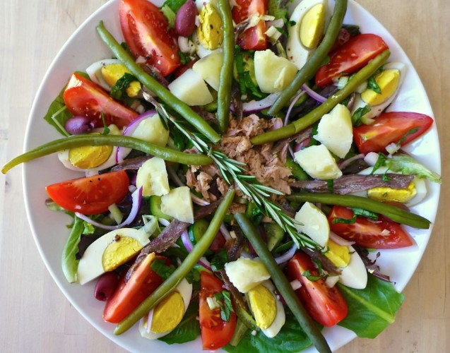
NIÇOISE SALAD (SALADA NISSARDA)

Niçoise salad (salade niçoise) is known throughout the world. Unfortunately, despite its success, the authentic and traditional Niçoise salad is only known by a minority of people.


The traditional recipe of Niçoise salad include tomato, hard boiled eggs, scallions, unpitted black olives and canned tuna or anchovies.
Prep Time: 15minutes mins
Cook Time: 10minutes mins
Total Time: 25minutes mins
Course: Salad
Cuisine: French
Servings: 6 people

Ingredients:
  • 100 g mesclun salad
  • 150 g tuna (solid, in olive oil), crumbled
  • 2 tomatoes , cut into wedges
  • 2 small cucumbers , sliced
  • 12 black olives (ideally small black olives from Nice)
  • 1 Mexican onion , finely chopped
  • ½ red onion , thinly sliced
  • 4 hard-boiled eggs , quartered
  • 6 fillets anchovy
  • ½ green pepper , thinly sliced
  • 100 g small fava beans , cooked
  • 1 clove garlic , halved
  • ½ sprig rosemary , finely chopped
  • 6 leaves basil , whole or cut in chiffonade
  • 6 tablespoons extra virgin olive oil
  • 2 tablespoons red wine vinegar
  • Salt
  • Pepper

Method:
  1. In a bowl, prepare a vinaigrette with the olive oil, vinegar, rosemary, salt and pepper.
  2. Rub a large plate with garlic.
  3. In the plate, place a bed of mesclun.
  4. Arrange tomatoes, boiled eggs, cucumbers, green peppers and tuna, anchovies, olives, spring onions, fava beans.
  5. Pour the vinaigrette on top and garnish with basil.

Reference:
https://www.196flavors.com/nicoise-salad-salada-nissarda/


Coq au Vin
Coq au vin is one of the most emblematic dishes of French gastronomy. It is a rooster cut into pieces and marinated in red wine. The meat is then braised and simmered for a long time in the wine.
It is accompanied by a garnish called “à la française” made up of small lardons, spring onions, button mushrooms and carrots. This garnish can sometimes contain buttered bread toast and flat parsley leaves.
The exact origin of coq au vin is unknown, but this recipe is full of legends. Its creation is nevertheless between the center and the east of the country. The commonly accepted legend of the origin of the coq au vin is in the Auvergne. The chief of the Arvernes tribe, the famous Vercingetorix would have sent a Gallic rooster to his enemy Julius Caesar who was besieging Gergovia in 52 BC. An episode that can be found in La guerre des Gaules.
Vercingetorix would have sent this rooster, symbol in the Gauls of fighting spirit and valour. Julius Caesar then proposed to Vercingetorix to come to dinner before the battle, he would have made him serve this rooster cooked in wine. The next day, Vercingetorix crushed the Roman armies.

Coq au vin is a French dish made with marinated rooster then braised in Burgundy wine and garnished with bacon bits, mushrooms and carrots.
Prep Time
1hour hr
Cook Time
3hours hrs
Resting Time
12hours hrs
Total Time
4hours hrs
Course: Main CourseCuisine: French Servings: 8 people Calories: 131kcal Author: Renards Gourmets
Ingredients
For the rooster and poultry stock
1 rooster , about 8 lb / 3.5 kg, cut into pieces (keep the carcass and fat)
1 bouquet garni
750 ml water
For the coq au vin marinade
800 ml full-bodied Burgundy red wine
4 juniper berries
1 clove
1 sprig thyme
2 bay leaves
For the toppings
250 g button mushrooms , cut
1,5 kg thin carrots , cut into thin sections
200 g smoked bacon , diced
2 sweet onions , peeled and finely diced
10 pearl onions
10 cloves garlic
For the sauce
300 ml veal stock
100 ml cognac
2 squares dark chocolate
Salt
Black pepper
Butter

Method:
  1. Flambé the pieces of rooster to remove any lingering fluff.
Marinade (to be prepared the day before)
Mix all the ingredients needed for the marinade in a bowl and add all the pieces of rooster except the carcass and the fat.
Leave to marinate in the fridge for 12 hours.
Poultry stock
In a Dutch oven (or cast iron pot), heat 2 tablespoons (30 g) of butter over medium heat and brown the carcass as well as the excess fat and skins.
Brown well for a few minutes, then cover with water.
Add the bouquet garni and, over medium to high heat, reduce the stock to half.
Using a cheesecloth, strain the broth well.
Pour it into a glass container and let it cool, then cover it and keep it in the fridge for 8 hours.
Cooking of the rooster
Take the rooster pieces out of the refrigerator and remove them from their marinade.
Reserve the marinade.
Using a cloth, dry the rooster pieces well.
Heat a large cast iron pot and sauté the diced bacon bits until golden brown.
Remove the pan from the heat, remove all the diced bacon bits and set them aside.
Place the pot over medium heat and brown the pieces of rooster skin side down in the fat from the bacon bits. If there is not enough fat, add 1 to 2 tablespoons (20 g) of butter if necessary.
Once the rooster pieces are golden brown, remove them from the pan and in the same fat, sauté the onions and 4 minced garlic cloves, stirring constantly, until golden brown.
Put the pieces of rooster back in the pot and immediately deglaze with cognac, and flambé everything.
Add the marinade liquid to the reserved wine, and add the reserved chicken stock until the pieces of rooster are covered.
Add the rest of the garlic cloves, unpeeled.
Cover and bring to a boil over medium to high heat.
As soon as it boils again, lower the heat and simmer over low heat for about 1 hour 30 minutes.
Uncover the pot and simmer again over low heat for 30 minutes to reduce the sauce.
During cooking, check the liquid level often and, if necessary, add the remaining chicken stock or, failing that, add boiling water.
Sauces and garnishes
After 2 hours of cooking, preheat the oven to 350 F (180°C), and place the pieces of rooster in a large baking dish (reserve the sauce).
Bake the pieces of rooster and roast them for 35 minutes or until the skin is crispy.
Meanwhile, in the pot, add the carrots, pearl onions, veal stock and dark chocolate.
Cover and cook over low to medium heat for 10 minutes.
Remove the lid and, stirring frequently, reduce over medium heat for 30 minutes or until the sauce is smooth.
Shortly before the end of cooking, in a frying pan, heat 1 tablespoon (15 g) of butter over high heat and sauté the mushrooms for a few minutes, stirring constantly.
Add the mushrooms and the diced bacon to the pan.
Season with salt and pepper.
Remove the coq au vin from the oven and add them to the pot.
Cook for 2 minutes.

Reference:
See on Authentic French Dishes
https://www.196flavors.com/hachis-parmentier/

MOST POPULAR

List of Classical Ballets

Art

Visual Studio code in Azure ML and Git

Study notes

VS code is a great tool to create and maintain applications, but it is as well a great too to manage Azure cloud resources fully integrated with GitHub.
It has a massive collection of extensions.
Last but very important: you can manage Kubernetes cluster from Docker and Azure. That the cherry on top so far because any deep learning experiment can be developed, tested and debugged locally.

PowerShell commands history
C:UsersUSER_NAMEAppDataRoamingMicrosoftWindowsPowerShellPSReadline

How to use it in Azure Machine learning - experiments (Data science)?

Requirements:
Install:
  • Visual studio code
  • Visual studio code extensions - mandatory:
    • Python
    • Jupiter
    • Azure Machine Learning
  • Visual studio code extensions - useful:
    • Polyglot Notebooks - https://marketplace.visualstudio.com/items?itemName=ms-dotnettools.dotnet-interactive-vscode
    • Remote SSH

Note before reading further.
If you have a fresh new install of VS Code, only on python kernel available, installed through VS Code then all may work somehow, I mean all except torch and Azure SDK
Otherwise:
Install Anaconda
Add all packages you need via conda (Anaconda navigator is really nice; need a good computer)
In VS Code select Python inconda environment
You will have all you ever need for any experiment and no problem with dependecies and pacjkages update.
In images (Docker or ACI) just keep simple; one pyton version and only packages you need via YAML file.


Upgrade pip (pip is a packages utility for python.
# In terminal run
python -m pip install -U pip

If you have not installed
# run in terminal or command windows prompt (as administrator)
# replace 19.1.1 with the last stable version, check https://pypi.org/project/pip/

python -m pip install downloads/pip-19.1.1-py2.py3-none-any.whl

#or
python -m pip install downloads/pip-19.1.1.tar.gz

#or
https://files.pythonhosted.org/packages/cb/28/91f26bd088ce8e22169032100d4260614fc3da435025ff389ef1d396a433/pip-20.2.4-py2.py3-none-any.whl -O ~/pip20.2.4 then do python -m pip install ~/pip20.2.4


Install basic python libraries used in Data Science (Azure ML)
pip install pandas
pip install numpy
pip install matplotlib
pip install scipy
pip install scikit-learn

Work with deep learning:
pip install torchvision
# if not, you may try
pip3 install torchvision

Just in case there are problems try this:
pip install --upgrade setuptools

Install python SDK
pip install azureml-core
pip install azure-ai-ml

Check:
pip list


Create first jupyter note.
Create a new file and give extension .ipynb
or
Use Command Palette (Ctrl+Shift+P) and run.
Create: New Jupyter Notebook

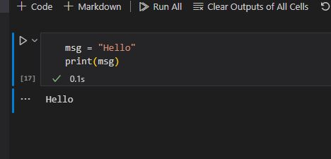
Write a test (python code) and run it.


To get data from Git or whatever other place you need wget utility.
In Linux you already have it.

On Windows and Mac OS:
Download it from https://www.gnu.org/software/wget/
Copy it (wget.exe) where you need ( do not leave it in downloads folder)
For example C:Wget or C:Program FilesWget (you must create Wget folder.

Add C:Wget in the Environment variable.
There are plenty of tutorials on the net, here there are two:
Windows - Command prompt: Windows CMD: PATH Variable - Add To PATH - Echo PATH - ShellHacks
Windows UI:How to Add to Windows PATH Environment Variable (helpdeskgeek.com)

Git / GitHub

Gits is part of anyone who run experiments.
Now VS Code fully integrate Git in UI

Install Git extension.

Basic operation:

1. Stage changes -> Click on + (right to added/changed/deleted file or on top line (Changes)
Write name of "Commit." and click "Commit"

2. Create Branch - 3 dots (very top)
Example "My New Branch"

3. Merge a branch to master:
- Click on 3 dots (very top)
- Select [Checkout to] and then the branch TO - master in this case
- Again 3 dots
- Click on [Branch] ->[Merge Branch] and then branch FROM - My New Branch, in this case
- Again 3 dots
- Select [Pull, Push] -> [Push]


Resources:
Working with Jupyter Notebooks in Visual Studio Code
Doing Data Science in Visual Studio Code
torch.nn — PyTorch 1.13 documentation


Machine Learning terms

Study notes

Data exploration and analysis
It is an iterative process- analyse data and test hypotheses.
  • Collect and clean data
  • Apply statistical techniques to better understand data.
  • Visualise data and determine relations.
  • Check hypotheses and repeat the process.

Statistics
Science of collecting and analysing numerical data in large quantities, especially for the purpose of inferring proportions in a whole from those in a representative sample
It is is fundamentally about taking samples of data and using probability functions to extrapolateinformation about the full population of data.

Statistic samples
Data we have "in hand", avilable to be analysed.

Statistics population
All possible data we could collect (theoretical).
We can wish to have data from population but that's may not be possible in timeframe and amiable resources. However, we must estimate labels with the sample we have.
Havin enough samples we can calculate the Probability Density Function

Probability Density Function
Estimate distribution of labels for the full population

Ensemble Algorithm
Works by combining multiple base estimators to produce an optimal model,

Bagging(Essamble alghorytm)
Technique used in ML training models - Regression.
Combine multiple base estimators to produce an optimal model by applying an aggregate function to base collection.

Boosting (Essamble alghorytm)
Technique used in ML training models - Regression.
Create a sequence of models that build on one another to improve predictive performance.


Jupiter notebook
Popular way to tun basic script in web browser (no need python installed to run)

NumPy
Python library that gives functionality comparable with tools like MATLABS and R.
Simplify analyzing and manipulating data.

Matplotlib
Provides attractive data visualizations

Panda
Python library for data analysis and manipulation (excel for Python) - easy to use functionality for data tables.
Simplify analyzing and manipulating data.
Include basic functionality for visualization (graphs)

TensorFlow
Open-source platform for machine learning (end to end)

SciKit-learn

Offers simple and effective predictive data analysis
TensorFlow Software library for machine learning and artificial intelligence - focus on training and inference of deep neural networks.
Supply machine learning and deep learning capabilities

predict()
Predicts the actual class.

predict_proba()
Predicts the class probabilities.

DataFrame
Data structure that organizes data into a 2-dimensional table of rows and columns, much like a spreadsheet.
One of the most common data structures used in modern data analytics because they are a flexible and intuitive way of storing and working with data.

pandas.DataFrame.to_dict()
Convert the DataFrame to a dictionary.
The type of the key-value pairs can be customized with the parameters which determines the type of the values of the dictionary.
  • ‘dict’ (default) :
    dict like {column -> {index -> value}}
  • ‘list’ :
    dict like {column -> [values]}
  • ‘series’ :
    dict like {column -> Series(values)}
  • ‘split’ :
    dict like {‘index’ -> [index], ‘columns’ -> [columns], ‘data’ -> [values]}
  • ‘tight’ :
    dict like {‘index’ -> [index], ‘columns’ -> [columns], ‘data’ -> [values], ‘index_names’ -> [index.names], ‘column_names’ -> [column.names]}
  • ‘records’ :
    list like [{column -> value}, … , {column -> value}]
  • ‘index’ :
    dict like {index -> {column -> value}}

Pecentile
Give you a number that describes the value that a given percent of the values are lower than.

Quantile
A cut point, or line of division, that splits a probability distribution into continuous intervals with equal probabilities
Eliminate all values that fall below a specific percentile

Probability distribution
A function that accepts as input elements of some specific set x∈X, and produces as output, real-valued numbers between 0 and 1.
A probability distribution is a statistical function that describes all the possible values and probabilities for a random variable within a given range.
This range will be bound by the minimum and maximum possible values, but where the possible value would be plotted on the probability distribution will be determined by a number of factors. The mean (average), standard deviation, skewness, and kurtosis of the distribution are among these factors.
https://www.simplilearn.com/tutorials/statistics-tutorial/what-is-probability-distribution

Normalize data
Process data so values retain their proportional distribution, but are measured on the same scale

Proportional distribution
Distribute values across considering other factors
Example: Department intends to distribute funds for employment services across all areas of the state taking into consideration population distribution and client needs.

Correlation measurement
Quantify the relationship between these columns.

Outlier
A data point that is noticeably different from the rest

Regression

Where models predict a number, establishing a relationship between variables in the data that represent characteristics - known as the feature - of the thing being observed, and the variable we're trying to predict—known as the label
Supervised machine learning techniques involve training a model to operate on a set of features(x1,x2...xn) and predict a label (y) using a dataset that includes some already-known label values.
Mathematical approach to find the relationship between two or more variables
Regression works by establishing a relationship between variables in the data that represent characteristics—known as the features—of the thing being observed, and the variable we're trying to predict—known as the label
https://learn.microsoft.com/en-us/training/modules/train-evaluate-regression-models/2-what-is-regression

Linear regression
Simplest form of regression, with no limit to the number of features used.
Comes in many forms - often named by the number of features used and the shape of the curve that fits.

Decision trees
Take a step-by-step approach to predicting a variable.
If we think of our bicycle example, the decision tree may be first split examples between ones that are during Spring/Summer and Autumn/Winter, make a prediction based on the day of the week. Spring/Summer-Monday may have a bike rental rate of 100 per day, while Autumn/Winter-Monday may have a rental rate of 20 per day.

Ensemble algorithms
Construct a large number of trees - allowing better predictions on more complex data.
Ensemble algorithms, such as Random Forest, are widely used in machine learning and science due to their strong prediction abilities.

Hyperparameters
For real life scenarios with complex models and big datasets a model must befit repentantly (train, compare, adjust, train and so on...)
Values that change the way that the model is fit during loops.
Hyperparameter example Learning rate = sets how much a model is adjusted every cycle.
learning_rate - hyperparameter of GradientBoostingRegressorestimator.
n_estimators - Hyperparameter of GradientBoostingRegressorestimator.
Type:
  • Discrete hyperparameter (select discrete values from continues distributions)
    • qNormal distribution
    • qUniformdistribution
    • qLognormal distribution
    • qLogUniform distribution
  • Continuous hyperparameters
    • Normal distribution
    • Uniform distribution
    • Lognormal distribution
    • LogUniform distribution

Normal distribution
Normal distribution or Gaussian distribution is a type of continuous probability distribution for a real-valued random variable

Uniform distribution
Continuous uniform distribution or rectangular distribution is a family of symmetric probability distributions. The distribution describes an experiment where there is an arbitrary outcome that lies between certain bounds.


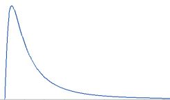
Lognormal distribution
Continuous probability distribution that models
right-skewed data.
The lognormal distribution is related to logs and the normal distribution.
LogUniform distribution
Continuous probability distribution. It is characterised by its probability density function, within the support of the distribution, being proportional to the reciprocal of the variable.

Preprocess the Data
Perform some preprocessing of the data to make it easier for the algorithm to fit a model to it.

Scaling numeric features
Normalizing numeric features so they're on the same scale prevents features with large values from producing coefficients that disproportionately affect the predictions.
Bring all features values between 0 & 1, Ex 3 => 0.3, 480 => 0.48, 65=> 0.65
they're on the same scale. This prevents features with large values from producing coefficients that disproportionately affect the predictions

Encoding categorical variables
Convert categorical features into numeric representations
S,M,L => 0.1.2
by using a one hot encoding technique you can create individual binary (true/false) features for each possible category value.

Hot Encoding categorical variables
S M L
1 0 0
0 1 0
0 0 1

Classification
Form of machine learning in which you train a model to predict which category an item belongs to

Binary classification
is classification with two categories.

Regularization
technique that reduces error from a model by avoiding overfitting and training the model to function properly.
helps us control our model capacity, ensuring that our models are better at making (correct) classifications on data points that they were not trained on, which we call the ability to generalize.
threshold
A threshold value of 0.5 is used to decide whether the predicted label is a 1 (P(y) > 0.5) or a 0 (P(y) <= 0.5).
You can use the predict_proba method to see the probability pairs for each case
If we were to change the threshold, it would affect the predictions; and therefore change the metrics in the confusion matrix.

pipeline

Used extensively in machine learning, often to mean very different things.
1. Allow to define set of preprocessing steps that end with an algorithm.
Then fit entire pipeline to the data => model encapsulate all preprocessing steps and the (regression) algorithm.


Classification algorithms
logistic regression algorithm, (linear algorithm)
Support Vector Machine algorithms: Algorithms that define a hyperplane that separates classes.
Tree-based algorithms: Algorithms that build a decision tree to reach a prediction
Ensemble algorithms: Algorithms that combine the outputs of multiple base algorithms to improve generalizability (ex Random Forest)

Multiclass classification
Combination of multiple binary classifiers

One vs Rest (OVR)
Multiclass classification classifier.
A classifier is created for each possible class value, with a positive outcome for cases where the prediction is this class, and negative predictions for cases where the prediction is any other class
Ex:
square or not
circle or not
triangle or not
hexagon or not

One vs One (OVO)
Multiclass classification classifier
a classifier for each possible pair of classes is created. The classification problem with four shape classes would require the following binary classifiers:
square or circle
square or triangle
square or hexagon
circle or triangle
circle or hexagon
triangle or hexagon

predict_proba
Returns probabilities of a classification label.
Example:
Have a trained classification model
May run confusion_matrix(y_test, predictions) - check result
Run y_score =model.predict_proba(X_tests)
We get probability of 0 or 1 for every record in X_test
[[0.81651727 0.18348273]
[0.96298333 0.03701667]
[0.80862083 0.19137917]
...
[0.60688422 0.39311578]
[0.10672996 0.89327004]
[0.63865894 0.36134106]]


Stratification technique
Used (example in classification) when splitting the data to maintain the proportion of each label value in the training and validation datasets.

Clustering
Clustering is a form of unsupervised machine learning in which observations are grouped into clusters based on similarities in their data values, or features
process of grouping objects with similar objects
‘unsupervised’ method, where ‘training’ is done without labels

MinMaxScaler
Normalize the numeric features so they're on the same scale.

#areaperimetercompactnesskernel_lengthkernel_widthasymmetry_coefficient


17111.5513.100.84555.1672.8456.715
5815.3814.770.88575.6623.4191.999

scaled_features = MinMaxScaler().fit_transform(features[data.columns[0:6]])
Result:
array([[0.44098206, 0.50206612, 0.5707804 , 0.48648649, 0.48610121,
0.18930164],
[0.40509915, 0.44628099, 0.66243194, 0.36880631, 0.50106914,
0.03288302],

fit(data)
Method is used to compute the mean and std dev for a given feature to be used further for scaling.

transform(data)
Method is used toperform scaling using mean and std dev calculated using the .fit() method.

fit_transform()
Method does both fits and transform.

Principal Component Analysis (PCA)
Analyze the relationships between the features and summarize each observation as coordinates for two principal components
Translate the N-dimensional feature values into two-dimensional coordinates.

Within cluster sum of squares (WCSS) metric often used to measure this tightness
Lower values meaning that the data points are closer

k-means clustering algorithm
Iterative algorithm that tries to partition the dataset into Kpre-defined distinct non-overlapping subgroups (clusters) where each data point belongs to only one group.
The way kmeans algorithm works is as follows:
• The feature values are vectorized to define n-dimensional coordinates (where n is the number of features). In the flower example, we have two features (number of petals and number of leaves), so the feature vector has two coordinates that we can use to conceptually plot the data points in two-dimensional space.
• You decide how many clusters you want to use to group the flowers, and call this value k. For example, to create three clusters, you would use a k value of 3. Then k points are plotted at random coordinates. These points will ultimately be the center points for each cluster, so they're referred to as centroids.
• Each data point (in this case flower) is assigned to its nearest centroid.
• Each centroid is moved to the center of the data points assigned to it based on the mean distance between the points.
• After moving the centroid, the data points may now be closer to a different centroid, so the data points are reassigned to clusters based on the new closest centroid.
• The centroid movement and cluster reallocation steps are repeated until the clusters become stable or a pre-determined maximum number of iterations is reached.

KMeans.inertia_
Sum of Squared errors (SSE)
Calculates the sum of the distances of all points within a cluster from the centroid of the point. It is the difference between the observed value and the predicted value.
The K-means algorithm aims to choose centroids that minimize the inertia, or within-cluster sum-of-squares criterion. Inertia can be recognized as a measure of how internally coherent clusters are.

PyTorch

PyTorch
Machine learning framework based on the Torch library, used for applications such as computer vision and natural language processing (NLP)
Supply machine learning and deep learning capabilities
An open source machine learning framework that accelerates the path from research prototyping to production deployment
PyTorch datasets - the data is stored in PyTorch *tensor* objects.

manual_seed(torch.manual_seed())
Sets the seed for generating random numbers.
Returns a torch.Generator object.

optimizer.zero_grad()
In PyTorch, for every mini-batch during the training phase, we typically want to explicitly set the gradients to zero before starting to do backpropragation (i.e., updating the Weights and biases) because PyTorch accumulates the gradients on subsequent backward passes.
Because of this, when you start your training loop, ideally you should zero out the gradients so that you do the parameter update correctly


Hierarchical Clustering
clustering algorithm in which clusters themselves belong to a larger group, which belong to even larger groups, and so on. The result is that data points can be clusters in differing degrees of precision: with a large number of very small and precise groups, or a small number of larger groups.
Useful for not only breaking data into groups, but understanding the relationships between these groups.
A major advantage of hierarchical clustering is that it does not require the number of clusters to be defined in advance, and can sometimes provide more interpretable results than non-hierarchical approaches.
The major drawback is that these approaches can take much longer to compute than simpler approaches and sometimes are not suitable for large datasets.

divisive method
Hierarchical Clustering
"top down" approach starting with the entire dataset and then finding partitions in a stepwise manner

agglomerative method
Hierarchical Clustering
"bottom up** approach. In this lab you will work with agglomerative clustering which roughly works as follows:
1. The linkage distances between each of the data points is computed.
2. Points are clustered pairwise with their nearest neighbor.
3. Linkage distances between the clusters are computed.
4. Clusters are combined pairwise into larger clusters.
5. Steps 3 and 4 are repeated until all data points are in a single cluster.

linkage function
Hierarchical Clustering - agglomerative method
can be computed in a number of ways:
• Ward linkage measures the increase in variance for the clusters being linked,
• Average linkage uses the mean pairwise distance between the members of the two clusters,
• Complete or Maximal linkage uses the maximum distance between the members of the two clusters.
Several different distance metrics are used to compute linkage functions:
• Euclidian or l2 distance is the most widely used. This metric is only choice for the Ward linkage method - measures of difference
• Manhattan or l1 distance is robust to outliers and has other interesting properties - measures of difference
• Cosine similarity, is the dot product between the location vectors divided by the magnitudes of the vectors. - measure of similarity
Similarity can be quite useful when working with data such as images or text documents.

Deep learning
Advanced form of machine learning that tries to emulate the way the human brain learns.
1. When the first neuron in the network is stimulated, the input signal is processed
2. If it exceeds a particular threshold, the neuron is activated and passes the signal on to the neurons to which it is connected.
3. These neurons in turn may be activated and pass the signal on through the rest of the network.
4. Over time, the connections between the neurons are strengthened by frequent use as you learn how to respond effectively.
Deep learning emulates this biological process using artificial neural networks that process numeric inputs rather than electrochemical stimuli.
The incoming nerve connections are replaced by numeric inputs that are typically identified as x (x1,x2…)
Associated with each x value is a weight (w)
Additionally, a bias (b) input is added to enable fine-grained control over the network
The neuron itself encapsulates a function that calculates a weighted sum of x, w, and b. This function is in turn enclosed in an activation function that constrains the result (often to a value between 0 and 1) to determine whether or not the neuron passes an output onto the next layer of neurons in the network.

Deep neural network
DNN model
The deep neural network model for the classifier consists of multiple layers of artificial neurons. In this case, there are four layers:
• An input layer with a neuron for each expected input (x) value.
• Two so-called hidden layers, each containing five neurons.
• An output layer containing three neurons - one for each class probability (y) value to be predicted by the model.
Particularly useful for dealing with data that consists of large arrays of numeric values - such as images.
Are the foundation for an area artificial intelligence called computer vision,

epochs
Training DNN model
The training process for a deep neural network consists of multiple iterations

backpropagation
Training DNN model
the loss from the model is calculated and used to adjust the weight and bias values

Calculating loss
Training DNN model
The loss is calculated using a function, which operates on the results from the final layer of the network, which is also a function
multiple observations, we typically aggregate the variance

Loss function
Training DNN model
the entire model from the input layer right through to the loss calculation is just one big nested function
Functions have a few really useful characteristics, including:
• You can conceptualize a function as a plotted line comparing its output with each of its variables.
• You can use differential calculus to calculate the derivative of the function at any point with respect to its variables.
The derivative of a function for a given point indicates whether the slope (or gradient) of the function output (in this case, loss) is increasing or decreasing with respect to a function variable (in this case, the weight value).
A positive derivative indicates that the function is increasing, and a negative derivative indicates that it is decreasing.

optimizer
apply this same trick for all of the weight and bias variables in the model and determine in which direction we need to adjust them (up or down) to reduce the overall amount of loss in the model.
There are multiple commonly used optimization algorithms:
- stochastic gradient descent (SGD),
- Adaptive Learning Rate (ADADELTA),
- Adaptive Momentum Estimation (Adam), and others;
All of which are designed to figure out how to adjust the weights and biases to minimize loss.

Learning rate
how much should the optimizer adjust the weights and bias values
A low learning rate results in small adjustments (so it can take more epochs to minimize the loss), while a high learning rate results in large adjustments (so you might miss the minimum altogether).

Convolutional neural networks (CNN)
A CNN typically works by extracting features from images, and then feeding those features into a fully connected neural network to generate a prediction.
CNNs consist of multiple layers, each performing a specific task in extracting features or predicting labels.
The feature extraction layers in the network have the effect of reducing the number of features from the potentially huge array of individual pixel values to a smaller feature set that supports label prediction.
1. An image is passed to the convolutional layer. In this case, the image is a simple geometric shape.
2. The image is composed of an array of pixels with values between 0 and 255 (for color images, this is usually a 3-dimensional array with values for red, green, and blue channels).
3. A filter kernel is generally initialized with random weights (in this example, we've chosen values to highlight the effect that a filter might have on pixel values; but in a real CNN, the initial weights would typically be generated from a random Gaussian distribution). This filter will be used to extract a feature map from the image data.
4. The filter is convolved across the image, calculating feature values by applying a sum of the weights multiplied by their corresponding pixel values in each position. A Rectified Linear Unit (ReLU) activation function is applied to ensure negative values are set to 0.
5. After convolution, the feature map contains the extracted feature values, which often emphasize key visual attributes of the image. In this case, the feature map highlights the edges and corners of the triangle in the image.

overlay
An image is also just a matrix of pixel values. To apply the filter, you "overlay" it on an image and calculate a weighted sum of the corresponding image pixel values under the filter kernel. The result is then assigned to the center cell of an equivalent 3x3 patch in a new matrix of values that is the same size as the image

Pooling layers
After extracting feature values from images, pooling (or downsampling) layers are used to reduce the number of feature values while retaining the key differentiating features that have been extracted.
One of the most common kinds of pooling is max pooling in which a filter is applied to the image, and only the maximum pixel value within the filter area is retained. So for example, applying a 2x2 pooling kernel to the following patch of an image would produce the result 155.
1. The feature map extracted by a filter in a convolutional layer contains an array of feature values.
2. A pooling kernel is used to reduce the number of feature values. In this case, the kernel size is 2x2, so it will produce an array with quarter the number of feature values.
3. The pooling kernel is convolved across the feature map, retaining only the highest pixel value in each position.

overfitting
the resulting model performs well with the training data but doesn't generalize well to new data on which it wasn't trained.
One technique you can use to mitigate overfitting is to include layers in which the training process randomly eliminates (or "drops") feature maps
Other techniques you can use to mitigate overfitting include randomly flipping, mirroring, or skewing the training images to generate data that varies between training epochs.
- For this reason, it’s common to use some kind of regularisation method to prevent the model from fitting too closely to the training data

Flattening layers
resulting feature maps are multidimensional arrays of pixel values. A flattening layer is used to flatten the feature maps into a vector of values that can be used as input to a fully connected layer.
CNN architecture 1. Images are fed into a convolutional layer. In this case, there are two filters, so each image produces two feature maps.
2. The feature maps are passed to a pooling layer, where a 2x2 pooling kernel reduces the size of the feature maps.
3. A dropping layer randomly drops some of the feature maps to help prevent overfitting.
4. A flattening layer takes the remaining feature map arrays and flattens them into a vector.
5. The vector elements are fed into a fully connected network, which generates the predictions. In this case, the network is a classification model that predicts probabilities for three possible image classes (triangle, square, and circle).

Transfer learning
Conceptually, this neural network consists of two distinct sets of layers:
1. A set of layers from the base model that perform feature extraction.
extraction layers apply convolutional filters and pooling to emphasize edges, corners, and other patterns in the images that can be used to differentiate them, and in theory should work for any set of images with the same dimensions as the input layer of the network
2. A fully connected layer that takes the extracted features and uses them for class prediction.
extraction layers apply convolutional filters and pooling to emphasize edges, corners, and other patterns in the images that can be used to differentiate them, and in theory should work for any set of images with the same dimensions as the input layer of the network
This approach enables you to keep the pre-trained weights for the feature extraction layers, which means you only need to train the prediction layers you have added.

Azure Machine Learning studio
Cloud-based service that helps simplify some of the tasks it takes to prepare data, train a model, and deploy a predictive service.

Azure Machine Learning workspace
Resource in your Azure subscription you use to manage data, compute resources, code, models, and other artifacts related to your machine learning workloads.

Azure Machine Learning compute
Cloud-based resources on which you can run model training and data exploration processes.
1. Compute Instances: Development workstations that data scientists can use to work with data and models.
2. Compute Clusters: Scalable clusters of virtual machines for on-demand processing of experiment code.
3. Inference Clusters: Deployment targets for predictive services that use your trained models.
4. Attached Compute: Links to existing Azure compute resources, such as Virtual Machines or Azure Databricks clusters.

Azure Machine Learning
Service for training and managing machine learning models, for which you need compute on which to run the training process.

Azure Automated Machine Learning
Automatically tries multiple pre-processing techniques and model-training algorithms in parallel.
These automated capabilities use the power of cloud compute to find the best performing supervised machine learning model for your data.
It provides a way to save time and resources by automating algorithm selection and hyperparameter tuning.

AutoML process
1. Prepare data: Identify the features and label in a dataset. Pre-process, or clean and transform, the data as needed.
2. Train model: Split the data into two groups, a training and a validation set. Train a machine learning model using the training data set. Test the machine learning model for performance using the validation data set.
3. Evaluate performance: Compare how close the model's predictions are to the known labels.
4. Deploy a predictive service: After you train a machine learning model, you can deploy the model as an application on a server or device so that others can use it.

Train model
You can use automated machine learning to train models for:
• Classification (predicting categories or classes)
• Regression (predicting numeric values)
• Time series forecasting (predicting numeric values at a future point in time)
In Automated Machine Learning, you can select configurations for the primary metric, type of model used for training, exit criteria, and concurrency limits.

Evaluate performance
After the job has finished you can review the best performing model.

Inference Clusters
Deployment targets for predictive services that use your trained models

Pipelines
Let you organize, manage, and reuse complex machine learning workflows across projects and users. A pipeline starts with the dataset from which you want to train the model

Components
Encapsulates one step in a machine learning pipeline

Azure Machine Learning Jobs
executes a task against a specified compute target

Stratified sampeling
technique used in Machine Learning to generate a test set
Random sampling is generally fine if the original dataset is large enough; if not, a bias is introduced due to the sampling error. Stratified Sampling is a sampling method that reduces the sampling error in cases where the population can be partitioned into subgroups.
We perform Stratified Sampling by dividing the population into homogeneous subgroups, called strata, and then applying Simple Random Sampling within each subgroup.
As a result, the test set is representative of the population, since the percentage of each stratum is preserved. The strata should be disjointed; therefore, every element within the population must belong to one and only one stratum.

ML experiment
• a named process, usually the running of a script or a pipeline, that can generate metrics and outputs and be tracked in the Azure Machine Learning workspace
• it can be run multiple times, with different data, code, or settings; and Azure Machine Learning tracks each run, enabling you to view run history and compare results for each run.
• When you submit an experiment, you use its run context to initialize and end the experiment run that is tracked in Azure Machine Learning
1. Every experiment generates log files (keep data between runs)
2. You can view the metrics logged by an experiment run in Azure Machine Learning studio or by using the RunDetails widget in a notebook
3. In addition to logging metrics, an experiment can generate output files. The output files of an experiment are saved in its outputs folder.

experiment script
• a Python code file that contains the code you want to run in the experiment
1. To access the experiment run context (which is needed to log metrics) the script must import the azureml.core.Run class and call its get_context method.
2. To run a script as an experiment, you must define
a. a script configuration that defines the script to be run and
b. the Python environment in which to run it.
This is implemented by using a ScriptRunConfig object.

Log experiment metrics
Run object
Every experiment generates log files that include the messages that would be written to the terminal during interactive execution.
If you want to record named metrics for comparison across runs, you can do so by using the Run object; which provides a range of logging functions specifically for this purpose. These include:
• log: Record a single named value.
• log_list: Record a named list of values.
• log_row: Record a row with multiple columns.
• log_table: Record a dictionary as a table.
• log_image: Record an image file or a plot.

Environment
Defines Python packages, environment variables, and Docker settings that are used in machine learning experiments, including in data preparation, training, and deployment to a web service.
An Environment is managed and versioned in an Azure Machine Learning Workspace.
You can update an existing environment and retrieve a version to reuse.
Environments are exclusive to the workspace they are created in and can't be used across different workspaces.
Azure Machine Learning provides curated environments, which are predefined environments that offer good starting points for building your own environments. Curated environments are backed by cached Docker images, providing a reduced run preparation cost.
Environment are created in by:
  • Initialize a new Environment object.
  • Use one of the Environment class methods: from_conda_specification, from_pip_requirements, or from_existing_conda_environment.
  • Use the submit method of the Experiment class to submit an experiment run without specifying an environment, including with an Estimator object.
argparse
To use parameters in a script, you must use a library such as argparse to read the arguments passed to the script and assign them to variables.

train_test_split sklearn
split model

LogisticRegression
Supervised classification algorithm.
The model builds a regression model to predict the probability that a given data entry belongs to the category numbered as “1” or "0"
Linear regression assumes that the data follows a linear function, Logistic regression models the data using the sigmoid function.

Hyperparameter
- configure how the model is trained
- top-level parameters that control the learning process and the model parameters that result from it. As a machine learning engineer designing a model, you choose and set hyperparameter values that your learning algorithm will use before the training of the model even begins

Regularization rate
(regression algorithm)
The Logistic regression function, which originally takes training data X, and label yas input, now needs to add one more input: the strength of regularization λ.
used to train models that generalize better on unseen data,by preventing the algorithm from overfitting the training dataset.

Hyperparameter
search space
Search space for hyperparameters values
To define a search space for hyperparameter tuning, create a dictionary with the appropriate parameter expression for each named hyperparameter
The specific values used in a hyperparameter tuning run depend on the type of sampling used.

Discrete hyperparameters
distributions
• qnormal
• quniform
• qlognormal
• qloguniform

Continuous hyperparameters
Distributions
• normal
• uniform
• lognormal
• loguniform

Hyperparameters search space
values sampling
Grid sampling - can only be employed when all hyperparameters are discrete, and is used to try every possible combination of parameters in the search space.
Random sampling is used to randomly select a value for each hyperparameter, which can be a mix of discrete and continuous values
Bayesian sampling chooses hyperparameter values based on the Bayesian optimization algorithm, which tries to select parameter combinations that will result in improved performance from the previous selection.

Training early termination
set an early termination policy that abandons runs that are unlikely to produce a better result than previously completed runs.
The policy is evaluated at an evaluation_interval you specify, based on each time the target performance metric is logged.
You can also set a delay_evaluation parameter to avoid evaluating the policy until a minimum number of iterations have been completed.

Data privacy parameters
The amount of variation caused by adding noise is configurable
epsilon This value governs the amount of additional risk that your personal data can be identified through rejecting the opt-out option and participating in a study
- A low epsilon value provides the most privacy, at the expense of less accuracy when aggregating the data
- A higher epsilon value results in aggregations that are more true to the actual data distribution, but in which the individual contribution of a single individual to the aggregated value is less obscured by noise - less privacy

Differential privacy
Technique that is designed to preserve the privacy of individual data points by adding "noise" to the data. The goal is to ensure that enough noise is added to provide privacy for individual values while ensuring that the overall statistical makeup of the data remains consistent, and aggregations produce statistically similar results as when used with the original raw data.

The noise is different for each analysis, so the results are non-deterministic – in other words, two analyses that perform the same aggregation may produce slightly different results.
The amount of variation caused by adding noise is configurable through a parameter called epsilon
  • A low epsilon value provides the most privacy, at the expense of less accuracy when aggregating the data.
  • A higher epsilon value results in aggregations that are more true to the actual data distribution, but in which the individual contribution of a single individual to the aggregated value is less obscured by noise.
SmartNoise
Create an analysis in which noise is added to the source data.
The underlying mathematics of how the noise is added can be quite complex, but SmartNoise takes care of most of the details for you.
  • Upper and lower bounds
    Clampingis used to set upper and lower bounds on values for a variable. This is required to ensure that the noise generated by SmartNoise is consistent with the expected distribution of the original data.
  • Sample size
    To generate consistent differentially private data for some aggregations, SmartNoise needs to know the size of the data sample to be generated.
  • Epsilon
    Put simplistically, epsilon is a non-negative value that provides an inverse measure of the amount of noise added to the data. A low epsilon results in a dataset with a greater level of privacy, while a high epsilon results in a dataset that is closer to the original data. Generally, you should use epsilon values between 0 and 1. Epsilon is correlated with another value named delta, that indicates the probability that a report generated by an analysis is not fully private.

Covariance
Establish relationships between variables.
Positive values - one feature increases, the second increases the same; direct relation.

Model explainers
Use statistical techniques to calculate feature importance.
Allow to quantify the relative influence each feature in the training dataset has on label prediction.
Explainers work by evaluating a test data set of feature cases and the labels the model predicts for them.

Global feature importance
quantifies the relative importance of each feature in the test dataset as a whole
It provides a general comparison of the extent to which each feature in the dataset influences prediction.

model-agnostic
Use ML models to study the the underlying structure without assuming that it can be accurately described by the model because of its nature.


Local feature importance
measures the influence of each feature value for a specific individual prediction.
For a regression model, there are no classes so the local importance values simply indicate the level of influence each feature has on the predicted scalar label.

MimicExplainer
Model explainers
An explainer that creates a global surrogate model that approximates your trained model and can be used to generate explanations.
This explainable model must have the same kind of architecture as your trained model (for example, linear or tree-based).

TabularExplainer
Model explainers
An explainer that acts as a wrapper around various SHAP explainer algorithms, automatically choosing the one that is most appropriate for your model architecture.

Model explainers
a Permutation Feature Importance explainer that analyzes feature importance by shuffling feature values and measuring the impact on prediction performance.

SHAP
SHapley Additive exPlanations — is probably the state of the art in Machine Learning explain ability.
In a nutshell, SHAP values are used whenever you have a complex model (could be a gradient boosting, a neural network, or anything that takes some features as input and produces some predictions as output) and you want to understand what decisions the model is making.

Disparity
a difference in level or treatment, especially one that is seen as unfair.
In prediction it is about fairness of the model

Measuring disparity in predictions
One way to start evaluating the fairness of a model is to compare predictions for each group within a sensitive feature.
To evaluate the fairness of a model, you can apply the same predictive performance metric to subsets of the data, based on the sensitive features on which your population is grouped, and measure the disparity in those metrics across the subgroups.
Potential causes of disparity • Data imbalance.
• Indirect correlation
• Societal biases.

Data imbalance
Some groups may be overrepresented in the training data, or the data may be skewed so that cases within a specific group aren't representative of the overall population.

Indirect correlation
The sensitive feature itself may not be predictive of the label, but there may be a hidden correlation between the sensitive feature and some other feature that influences the prediction. For example, there's likely a correlation between age and credit history, and there's likely a correlation between credit history and loan defaults. If the credit history feature is not included in the training data, the training algorithm may assign a predictive weight to age without accounting for credit history, which might make a difference to loan repayment probability.

Societal biases
Subconscious biases in the data collection, preparation, or modeling process may have influenced feature selection or other aspects of model design.

Fairlearn
Python package that you can use to analyze models and evaluate disparity between predictions and prediction performance for one or more sensitive features.
The mitigation support in Fairlearn is based on the use of algorithms to create alternative models that apply parity constraints to produce comparable metrics across sensitive feature groups. Fairlearn supports the following mitigation techniques.

Exponentiated Gradient
Fairlearn techniques
A reduction technique that applies a cost-minimization approach to learning the optimal trade-off of overall predictive performance and fairness disparity
- Binary classification
- Regression

Grid Search
Fairlearn techniques
A simplified version of the Exponentiated Gradient algorithm that works efficiently with small numbers of constraints
- Binary classification
- Regression

Threshold Optimizer
Fairlearn techniques
A post-processing technique that applies a constraint to an existing classifier, transforming the prediction as appropriate
- Binary classification

Fairlearn constraints
• Demographic parity
Use this constraint with any of the mitigation algorithms to minimize disparity in the selection rate across sensitive feature groups. For example, in a binary classification scenario, this constraint tries to ensure that an equal number of positive predictions are made in each group.
• True positive rate parity:
Use this constraint with any of the mitigation algorithms to minimize disparity in true positive rate across sensitive feature groups. For example, in a binary classification scenario, this constraint tries to ensure that each group contains a comparable ratio of true positive predictions.
• False-positive rate parity:
Use this constraint with any of the mitigation algorithms to minimize disparity in false_positive_rate across sensitive feature groups. For example, in a binary classification scenario, this constraint tries to ensure that each group contains a comparable ratio of false-positive predictions.
• Equalized odds:
Use this constraint with any of the mitigation algorithms to minimize disparity in combined true positive rate and false_positive_rate across sensitive feature groups. For example, in a binary classification scenario, this constraint tries to ensure that each group contains a comparable ratio of true positive and false-positive predictions.
• Error rate parity:
Use this constraint with any of the reduction-based mitigation algorithms (Exponentiated Gradient and Grid Search) to ensure that the error for each sensitive feature group does not deviate from the overall error rate by more than a specified amount.
• Bounded group loss:
Use this constraint with any of the reduction-based mitigation algorithms to restrict the loss for each sensitive feature group in a regression model.

data drift
change in data profiles between training and inferencing and over the time.
To monitor data drift using registered datasets, you need to register two datasets:
- A baseline dataset - usually the original training data.
- A target dataset that will be compared to the baseline based on time intervals. This dataset requires a column for each feature you want to compare, and a timestamp column so the rate of data drift can be measured.

Service tags
a group of IP address prefixes from a given Azure service
Microsoft manages the address prefixes encompassed by the service tag and automatically updates the service tag as addresses change, minimizing the complexity of frequent updates to network security rules.
You can use service tags in place of specific IP addresses when you create security rules to define network access controls on network security groups or Azure Firewall.

Azure VNet
the fundamental building block for your private network in Azure. VNet enables Azure resources, such as Azure Blob Storage and Azure Container Registry, to securely communicate with each other, the internet, and on-premises networks.
With a VNet, you can enhance security between Azure resources and filter network traffic to ensure only trusted users have access to the network.

IP address space:
When creating a VNet, you must specify a custom private IP address space using public and private (RFC 1918) addresses.

Subnets
enable you to segment the virtual network into one or more sub-networks and allocate a portion of the virtual network's address space to each subnet, enhancing security and performance.

Network interfaces (NIC)
the interconnection between a VM and a virtual network (VNet). When you create a VM in the Azure portal, a network interface is automatically created for you.

Network security groups (NSG)
can contain multiple inbound and outbound security rules that enable you to filter traffic to and from resources by source and destination IP address, port, and protocol.

Load balancers
can be configured to efficiently handle inbound and outbound traffic to VMs and VNets, while also offering metrics to monitor the health of VMs.

Service endpoints
provide the identity of your virtual network to the Azure service.
Service endpoints use public IP addresses
Once you enable service endpoints in your virtual network, you can add a virtual network rule to secure the Azure service resources to your virtual network.

Private endpoints
effectively bringing the Azure services into your VNet
Private endpoint uses a private IP address from your VNet
network interfaces that securely connect you to a service powered by Azure Private Link

Private Link Service
your own service, powered by Azure Private Link that runs behind an Azure Standard Load Balancer, enabled for Private Link access. This service can be privately connected with and consumed using Private Endpoints deployed in the user's virtual network

Azure VPN gateway
Connects on-premises networks to the VNet over a private connection. Connection is made over the public internet. There are two types of VPN gateways that you might use:
• Point-to-site: Each client computer uses a VPN client to connect to the VNet.
• Site-to-site: A VPN device connects the VNet to your on-premises network.

ExpressRoute
Connects on-premises networks into the cloud over a private connection. Connection is made using a connectivity provider.

Azure Bastion
In this scenario, you create an Azure Virtual Machine (sometimes called a jump box) inside the VNet. You then connect to the VM using Azure Bastion. Bastion allows you to connect to the VM using either an RDP or SSH session from your local web browser. You then use the jump box as your development environment. Since it is inside the VNet, it can directly access the workspace.

Azure Databricks
Microsoft analytics service, part of the Microsoft Azure cloud platform. It offers an integration between Microsoft Azure and the Apache Spark's Databricks implementation

notebook
a document that contains runnable code, descriptive text, and visualizations.
We can override the default language by specifying the language magic command %<language> at the beginning of a cell.
The supported magic commands are:
• %python
• %r
• %scala
• %sql
Notebooks also support a few auxiliary magic commands:
• %sh: Allows you to run shell code in your notebook
• %fs: Allows you to use dbutils filesystem commands
• %md: Allows you to include various types of documentation, including text, images, and mathematical formulas and equations.


workspace
It groups objects (like notebooks, libraries, experiments) into folders,
Provides access to your data,
Provides access to the computations resources used (clusters, jobs).

cluster
set of computational resources on which you run your code (as notebooks or jobs). We can run ETL pipelines, or machine learning, data science, analytics workloads on the cluster.
• An all-purpose cluster. Multiple users can share such clusters to do collaborative interactive analysis.
• A jbto run a specific job. The cluster will be terminated when the job completes (A job is a way of running a notebook or JAR either immediately or on a scheduled basis).

job
a way of running a notebook or JAR either immediately or on a scheduled basis

Databricks runtimes
the set of core components that run on Azure Databricks clusters.
Azure Databricks offers several types of runtimes:
Databricks Runtime: includes Apache Spark, components and updates that optimize the usability, performance, and security for big data analytics.
Databricks Runtime for Machine Learning: a variant that adds multiple machine learning libraries such as TensorFlow, Keras, and PyTorch.
Databricks Light: for jobs that don’t need the advanced performance, reliability, or autoscaling of the Databricks Runtime.

Azure Databricks database
a collection of tables. An Azure Databricks table is a collection of structured data.
We can cache, filter, and perform any operations supported by Apache Spark DataFrames on Azure Databricks tables. We can query tables with Spark APIs and Spark SQL.

Databricks File System (DBFS)
distributed file system mounted into a Databricks workspace and available on Databricks clusters. DBFS is an abstraction on top of scalable object storage and offers the following benefits:
• Allows you to mount storage objects so that you can seamlessly access data without requiring credentials.
• Allows you to interact with object storage using directory and file semantics instead of storage URLs.
• Persists files to object storage, so you won’t lose data after you terminate a cluster.

Resilient Distributed Dataset (RDD)
The fundamental data structure of Apache Spark which are an immutable collection of objects which computes on the different node of the cluster.
Each and every dataset in Spark RDD is logically partitioned across many servers so that they can be computed on different nodes of the cluster.

MLLib
SAME LIBRARY as Spark ML
legacy approach for machine learning on Apache Spark. It builds off of Spark's Resilient Distributed Dataset (RDD) data structure.
additional data structures on top of the RDD, such as DataFrames, have reduced the need to work directly with RDDs.
classic" MLLib namespace is org.apache.spark.mllib

Spark ML
SAME LIBRARY as MLLib
Primary library for machine learning development in Apache Spark.
It supports DataFrames in its API (versus the classic RDD approach).
USE this as much as you can This makes Spark ML an easier library to work with for data scientists .
As Spark DataFrames share many common ideas with the DataFrames used in Pandas and R.
Spark ML workspace is org.apache.spark.ml.

Train and validate a model
The process of training and validating a machine learning model using Spark ML is fairly straightforward. The steps are as follows:
• Splitting data.
• Training a model.
• Validating a model.

Splitting data
splitting data between training and validation datasets
This hold-out dataset can be useful for determining whether the training model is overfitting
DataFrames support a randomSplit() method, which makes this process of splitting data simple

Training a model
Training a model relies on three key abstractions:
• a transformer - performing feature engineering and feature selection, as the result of a transformer is another DataFrame - support a randomSplit()
• an estimator - takes a DataFrame as an input and returns a model. It takes a DataFrame as an input and returns a model, which is itself a transformer.
ex: LinearRegression
It accepts a DataFrame and produces a Model. Estimators implement a .fit() method.
• a pipeline - combine together estimators and transformers and implement a .fit()

Validating a model
process based on built-in summary statistics
the model contains a summary object, which includes scores such as Root Mean Square Error (RMSE), Mean Absolute Error (MAE), and coefficient of determination (R2, pronounced R-squared)
with a validation dataset, it is possible to calculate summary statistics on a never-before-seen set of data, running the model's transform() function against the validation dataset.

other machine learning frameworks
Azure Databricks supports machine learning frameworks other than Spark ML and MLLib.
For libraries, which do not support distributed training, it is also possible to use a single node cluster. For example, PyTorch and TensorFlow both support single node use.

DataFrames
the distributed collections of data, organized into rows and columns. Each column in a DataFrame has a name and an associated type.
Spark DataFrames can be created from various sources, such as CSV files, JSON, Parquet files, Hive tables, log tables, and external databases.

Query dataframes
Spark SQL is a component that introduced the DataFrames, which provides support for structured and semi-structured data.
Spark has multiple interfaces (APIs) for dealing with DataFrames:
• the .sql() method, which allows to run arbitrary SQL queries on table data.
• use the Spark domain-specific language for structured data manipulation, available in Scala, Java, Python, and R.

DataFrame API
The Apache Spark DataFrame API provides a rich set of functions (select columns, filter, join, aggregate, and so on) that allow you to solve common data analysis problems efficiently. A complex operation where tables are joined, filtered, and restructured is easy to write, easy to understand, type safe, feels natural for people with prior sql experience
statistics about the DataFrame • Available statistics are:
• Count
• Mean
• Stddev
• Min
• Max
• Arbitrary approximate percentiles specified as a percentage (for example, 75%).

Plot options
• The following display options are available:
• We can choose the DataFrame columns to be used as axes (keys, values).
• We can choose to group our series of data.
• We can choose the aggregations to be used with our grouped data (avg, sum, count, min, max).

Machine learning
Data science technique used to extract patterns from data allowing computers to identify related data, forecast future outcomes, behaviors, and trends.
In machine learning, you train the algorithm with data and answers, also known as labels, and the algorithm learns the rules to map the data to their respective labels.

Synthetic Minority Over-sampling Technique (SMOTE)
Oversampling technique that allows us to generate synthetic samples for our minority categories
the idea is based on the K-Nearest Neighbors algorithm
We get a difference between a sample and one of its k nearest neighbours and multiply by some random value in the range of (0, 1). Finally, we generate a new synthetic sample by adding the value we get from the previous operation

Imputation of null values
Null values refer to unknown or missing data. Strategies for dealing with this scenario include:
• Dropping these records: Works when you do not need to use the information for downstream workloads.
• Adding a placeholder (for example, -1): Allows you to see missing data later on without violating a schema.
• Basic imputing: Allows you to have a "best guess" of what the data could have been, often by using the mean or median of non-missing data for numerical data type, or most_frequent value of non-missing data for categorical data type.
• Advanced imputing: Determines the "best guess" of what data should be using more advanced strategies such as clustering machine learning algorithms or oversampling techniques such as SMOTE (Synthetic Minority Over-sampling Technique).

ScriptRunConfig
To submit a run, create a configuration object that describes how the experiment is run. ScriptRunConfig is an examples of configuration objects used.
Identifies the Python script file to be run in the experiment. An experiment can be run based on it.
The ScriptRunConfig also determines the compute target and Python environment.

data cleaning
Imputation of null values, Imputation of null values, Duplicate records, Outliers

feature engineering
process of generating new predictive features from existing raw data
it is important to derive features from existing raw data that better represent the nature of the data and thus help improve the predictive power of the machine learning algorithms
• Aggregation (count, sum, average, mean, median, and the like)
• Part-of (year of date, month of date, week of date, and the like)
• Binning (grouping entities into bins and then applying aggregations)
• Flagging (boolean conditions resulting in True of False)
• Frequency-based (calculating the frequencies of the levels of one or more categorical variables)
• Embedding (transforming one or more categorical or text features into a new set of features, possibly with a different cardinality)
• Deriving by example

data scaling
Bring features to similar scales
There are two common approaches to scaling numerical features:
• Normalization - mathematically rescales the data into the range [0, 1].
• Standardization - rescales the data to have mean = 0 and standard deviation = 1
For the numeric input
- compute the mean and standard deviation using all the data available in the training dataset.
- then for each individual input value, you scale that value by subtracting the mean and then dividing by the standard deviation.

data encoding
converting data into a format required for a number of information processing needs
We will look at two common approaches for encoding categorical data:
• Ordinal encoding - converts categorical data into integer codes ranging from 0 to (number of categories – 1).
• One-hot encoding - transforming each categorical value into n (= number of categories) binary values, with one of them 1, and all others 0 (recommended)

MLflow
Open-source product designed to manage the Machine Learning development lifecycle.
Allows data scientists to train models, register those models, deploy the models to a web server, and manage model updates.
Important part of machine learning with Azure Databricks, as it integrates key operational processes with the Azure Databricks interface (also operate on workloads outside of Azure Databricks)
Offers a standardized format for packaging models for distribution.
Components:
• MLflow Tracking - provides the ability to audit the results of prior model training executions. It is built around runs
• MLflow Projects - a way of packaging up code in a manner, which allows for consistent deployment and the ability to reproduce results
• MLflow Models - standardized model format allows MLflow to work with models generated from several popular libraries, including scikit-learn, Keras, MLlib, ONNX, and more
• MLflow Model Registry - llows data scientists to register models in a registry
Key steps:
• Mode registration - stores the details of a model in the MLflow Model Registry, along with a name for ease of access
• Model Versioning - makes model management easy by labeling new versions of models and retaining information on prior model versions automatically

MLflow Tracking
To use MLflow to track metrics for an inline experiment, you must set the MLflow tracking URI to the workspace where the experiment is being run. This enables you to use mlflow tracking methods to log data to the experiment run.
When you use MLflow tracking in an Azure ML experiment script, the MLflow tracking URI is set automatically when you start the experiment run. However, the environment in which the script is to be run must include the required mlflow packages.
It is built around runs, that is, executions of code for a data science task. Each run contains several key attributes, including:
  • Parameters:
    Key-value pairs, which represent inputs. Use parameters to track hyperparameters, that is, inputs to functions, which affect the machine learning process.
  • Metrics:
    Key-value pairs, which represent how the model is performing. This can include evaluation measures such as Root Mean Square Error, and metrics can be updated throughout the course of a run. This allows a data scientist, for example, to track Root Mean Square Error for each epoch of a neural network.
  • Artifacts:
    Output files. Artifacts may be stored in any format, and can include models, images, log files, data files, or anything else, which might be important for model analysis and understanding.
Experiments
Intended to collect and organize runs
The data scientist can then review the individual runs in order to determine which run generated the best model.

Run
Single trial of an experiment.
Object is used to monitor the asynchronous execution of a trial, log metrics and store outputof the trial, and to analyze results and access artifacts generated by the trial.
Used inside of your experimentation code to log metrics and artifacts to the Run History service.
Used outsideof your experiments tomonitor progress and to query and analyzethe metrics and results that were generated.
Functionality of Run:
  • Storing and retrieving metrics and data
  • Uploading and downloading files
  • Using tags as well as the child hierarchy for easy lookup of past runs
  • Registering stored model files as a model that can be operationalized
  • Storing, modifying, and retrieving properties of a run
  • Loading the current run from a remote environment with the get_context method
  • Efficiently snapshotting a file or directory for reproducibility
MLflow Projects
A project in MLflow is a method of packaging data science code. This allows other data scientists or automated processes to use the code in a consistent manner.
Each project includes at least one entry point, which is a file (either .py or .sh)
Projects also specify details about the environment.

MLflow Models
A model in MLflow is a directory containing an arbitrary set of files along with an MLmodel file in the root of the directory.
Each model has a signature, which describes the expected inputs and outputs for the model.
allows models to be of a particular flavor, which is a descriptor of which tool or library generated a model. This allows MLflow to work with a wide variety of modeling libraries, such as scikit-learn, Keras, MLlib, ONNX, and many

MLflow Model Registry
The MLflow Model Registry allows a data scientist to keep track of a model from MLflow Models
the data scientist registers a model with the Model Registry, storing details such as the name of the model. Each registered model may have multiple versions, which allow a data scientist to keep track of model changes over time.
t is also possible to stage models. Each model version may be in one stage, such as Staging, Production, or Archived. Data scientists and administrators may transition a model version from one stage to the next.

DatabricksStep
specialized pipeline step supported by Azure Machine Learning (Azure Data bricks), with which you can run a notebook, script, or compiled JAR on an Azure Databricks cluster
In order to run a pipeline step on a Databricks cluster, you need to do the following steps:
1. Attach Azure Databricks Compute to Azure Machine Learning workspace.
2. Define DatabricksStep in a pipeline.
3. Submit the pipeline.

Real-Time Inferencing
The model is deployed as part of a service that enables applications to request immediate, or real-time, predictions for individual, or small numbers of data observations.
In Azure Machine learning, you can create real-time inferencing solutions by deploying a model as a real-time service, hosted in a containerized platform such as Azure Kubernetes Services (AKS)
You can use the service components and tools to register your model and deploy it to one of the available compute targets so it can be made available as a web service in the Azure cloud, or on an IoT Edge device:

targets
1. Local web service - Testing/debug - Good for limited testing and troubleshooting.
2. Azure Kubernetes Service (AKS) - Real-time inference - Good for high-scale production deployments. Provides autoscaling, and fast response times.
3. Azure Container Instances (ACI) - Testing - Good for low scale, CPU-based workloads.
4. Azure Machine Learning Compute Clusters - Batch inference - Run batch scoring on serverless compute. Supports normal and low-priority VMs.
5. Azure IoT Edge - (Preview) IoT module - Deploy & serve ML models on IoT devices.

Deploy a model to Azure ML
To deploy a model as an inferencing webservice, you must perform the following tasks:
1. Register a trained model.
2. Define an Inference Configuration.
3. Define a Deployment Configuration.
4. Deploy the Model.

Hyperparameter tuning the process of choosing the hyperparameter that has the best result on our loss function, or the way we penalize an algorithm for being wrong.
Within Azure Databricks, there are two approaches to tune hyperparameters, which will be discussed in the next units:
• Automated MLflow tracking - common and simple approach to track model training in Azure Databricks
• Hyperparameter tuning with Hyperopt.
k-fold cross-validation A model is then trained on k-1 folds of the training data and the last fold is used to evaluate its performance.

automated MLflow Tracking
When you use automated MLflow for model tuning, the hyperparameter values and evaluation metrics are automatically logged in MLflow and a hierarchy will be created for the different runs that represent the distinct models you train.
To use automated MLflow tracking, you have to do the following:
1. Use a Python notebook to host your code.
2. Attach the notebook to a cluster with Databricks Runtime or Databricks Runtime for Machine Learning.
3. Set up the hyperparameter tuning with CrossValidator or TrainValidationSplit.

Hyperopt
tool that allows you to automate the process of hyperparameter tuning and model selection
Hyperopt is simple to use, but using it efficiently requires care. The main advantage to using Hyperopt is that it is flexible and it can optimize any Python model with hyperparameters
Hyperopt is already installed if you create a compute with the Databricks Runtime ML. To use it when training a Python model, you should follow these basic steps:
1. Define an objective function to minimize.
2. Define the hyperparameter search space.
3. Specify the search algorithm.
4. Run the Hyperopt function fmin().
objective function represents what the main purpose is of training multiple models through hyperparameter tuning. Often, the objective is to minimize training or validation loss.

hyperparameter search algorithm
There are two main choices in how Hyperopt will sample over the search space:
1. hyperopt.tpe.suggest: Tree of Parzen Estimators (TPE), a Bayesian approach, which iteratively and adaptively selects new hyperparameter settings to explore based on past results.
2. hyperopt.rand.suggest: Random search, a non-adaptive approach that samples over the search space.

Horovod
help data scientists when training deep learning models.
allows data scientists to distribute the training process and make use of Spark's parallel processing.
is designed to take care of the infrastructure management so that data scientists can focus on training models.

HorovodRunner
is a general API, which triggers Horovod jobs. The benefit of using HorovodRunner instead of the Horovod framework directly, is that HorovodRunner has been designed to distribute deep learning jobs across Spark workers.
->HorovodRunner is more stable for long-running deep learning training jobs on Azure Databricks.
Before working with Horovod and HorovodRunner, the code used to train the deep learning model should be tested on a single-node cluster

Petastorm
library that enables single machine or distributed training and evaluation of deep learning models from datasets in Apache Parquet format. It supports ML frameworks such as Tensorflow, Pytorch, and PySpark and can be used from pure Python code.

LinearRegression
In Scikit-Learn, training algorithms are encapsulated in estimators, and in this case we'll use the LinearRegression estimator to train a linear regression model.

Authentication with Azure AD
• Interactive:
You use your account in Azure Active Directory to either manually authenticate or obtain an authentication token. Interactive authentication is used during experimentation and iterative development. It enables you to control access to resources (such as a web service) on a per-user basis.
• Service principal:
You create a service principal account in Azure Active Directory, and use it to authenticate or obtain an authentication token. A service principal is used when you need an automated process to authenticate to the service. For example, a continuous integration and deployment script that trains and tests a model every time the training code changes needs ongoing access and so would benefit from a service principal account.
• Azure CLI session:
You use an active Azure CLI session to authenticate. Azure CLI authentication is used during experimentation and iterative development, or when you need an automated process to authenticate to the service using a pre-authenticated session. You can log in to Azure via the Azure CLI on your local workstation, without storing credentials in code or prompting the user to authenticate.
• Managed identity:
When using the Azure Machine Learning SDK on an Azure Virtual Machine, you can use a managed identity for Azure. This workflow allows the VM to connect to the workspace using the managed identity, without storing credentials in code or prompting the user to authenticate. Azure Machine Learning compute clusters can also be configured to use a managed identity to access the workspace when training models.

Service principal
Object that defines what the app can actually do in the specific tenant, who can access the app, and what resources the app can access.
When an application is given permission to access resources in a tenant (upon registration or consent), a service principal object is created
A service principal is used when you need an automated process to authenticate to the service.
For example, a continuous integration and deployment script that trains and tests a model every time the training code changes needs ongoing access and so would benefit from a service principal account.

Managed Identities
Managed identities allow you to authenticate services by providing an automatically managed identity for applications or services to use when connecting to Azure cloud services.
Managed identities work with any service that supports Azure AD authentication, and provides activity logs so admins can see user activity such as log-in times, when operations were started, and by whom.
Main resources
Exam DP-100: Designing and Implementing a Data Science Solution on Azure - Certifications | Microsoft Learn
Welcome to Python.org
NumPy user guide — NumPy v1.24 Manual
Introduction to Tensors | TensorFlow Core
pandas - Python Data Analysis Library (pydata.org)
All things · Deep Learning (dzlab.github.io)
API reference — pandas 1.5.3 documentation (pydata.org)
Track ML experiments and models with MLflow - Azure Machine Learning | Microsoft Learn
Lognormal Distribution: Uses, Parameters & Examples - Statistics By Jim
Normal Distribution | Examples, Formulas, & Uses (scribbr.com)

Lab hands-on Numpy and Pandas

Study notes

numpy.array
create an array of items optimised for data analysis.
import numpy as np

# Data loaded into a Python list structure
data = [50,50,47,97,49,3,53,42,26,74,82,62,37]

# Data is optimised for numeric analysis
val = np.array(data)

print (type(data),'x 2:', data * 2)
print (type(val),'x 2:', grades * 2)

Result:
<class 'list'> x 2: [50, 50, 47, 97, 49, 3, 53, 42, 26, 74, 82, 62, 37, 50, 50, 47, 97, 49, 3, 53, 42, 26, 74, 82, 62, 37]
<class 'numpy.ndarray'> x 2: [100 100 94 194 98 6 106 84 52 148 164 124 74]


numpy.shape
Return shape of an array

np.shape(val)
# or
val.shape

Result:
(13,)
13 elements (one dimension aray)

numpy.mean()
Return arithmetic mean (average)

import numpy as np

data = [50,50,47,97,49,3,53,42,26,74]
val = np.array(data)

val.mean()

Result:
49.1

Display numpay array.

import numpy as np

data = [50,50,47,97,49,3,53,42,26,74,82,62,37,15,70,27,36,35,48,52,63,64]grades = np.array(data)
study_hours = [10.0,11.5,9.0,16.0,9.25,1.0,11.5,9.0,8.5,14.5,15.5,13.75,9.0,8.0,15.5,8.0,9.0,6.0,10.0,12.0,12.5,12.0]

student_data = np.array([study_hours, grades])
print(student_data)student_data

Result:
[[10. 11.5 9. 16. 9.25 1. 11.5 9. 8.5 14.5 15.5 13.75
9. 8. 15.5 8. 9. 6. 10. 12. 12.5 12. ]
[50. 50. 47. 97. 49. 3. 53. 42. 26. 74. 82. 62.
37. 15. 70. 27. 36. 35. 48. 52. 63. 64. ]]
array([[10. , 11.5 , 9. , 16. , 9.25, 1. , 11.5 , 9. , 8.5 ,
14.5 , 15.5 , 13.75, 9. , 8. , 15.5 , 8. , 9. , 6. ,
10. , 12. , 12.5 , 12. ],
[50. , 50. , 47. , 97. , 49. , 3. , 53. , 42. , 26. ,
74. , 82. , 62. , 37. , 15. , 70. , 27. , 36. , 35. ,
48. , 52. , 63. , 64. ]])


Format output of a float number
Set number of decimals to be shown after decimal point
import numpy as np

data = [50,50,47,97,49,3,53,42,26,74,82,62,37,15,70,27,36,35,48,52,63,64]grades = np.array(data)
study_hours = [10.0,11.5,9.0,16.0,9.25,1.0,11.5,9.0,8.5,14.5,15.5,13.75,9.0,8.0,15.5,8.0,9.0,6.0,10.0,12.0,12.5,12.0]

avg_study = student_data[0].mean()
avg_grade = student_data[1].mean()

# avg_study value will go into the first {:.2f} and the avg_grade value will go into the second
# {:.2f} mans value will be shown as float number with 2 fingers after decimal point and as many as necessary before decimal point.
print('Average study hours: {:.2f}Average grade: {:.2f}'.format(avg_study, avg_grade))

Result:
Average study hours: 10.52
Average grade: 49.18

Multidimensional numpy array
import numpy as np

data = [50,50,47,97,49,3,53,42,26,74,82,62,37,15,70,27,36,35,48,52,63,64]
grades = np.array(data)

study_hours = [10.0,11.5,9.0,16.0,9.25,1.0,11.5,9.0,8.5,14.5,15.5,
13.75,9.0,8.0,15.5,8.0,9.0,6.0,10.0,12.0,12.5,12.0]

name = ['Dan', 'Joann', 'Pedro', 'Rosie', 'Ethan', 'Vicky', 'Frederic', 'Jimmie',
'Rhonda', 'Giovanni', 'Francesca', 'Rajab', 'Naiyana', 'Kian', 'Jenny',
'Jakeem','Helena','Ismat','Anila','Skye','Daniel','Aisha']

student_data = np.array([name, study_hours, grades])

student_data.shape

Result:
(3,22)
3 arrays, each with 22 elements.

Panda dataframe
Numpy manages perfect unidimensional data. Pandas is used to manipulate multidimensional data. It uses dataframes.

import pandas as pd

grades = [50,50,47,97,49,3,53,42,26,74,82,62,37,15,70,27,36,35,48,52,63,64]
study_hours = [10.0,11.5,9.0,16.0,9.25,1.0,11.5,9.0,8.5,14.5,15.5,
13.75,9.0,8.0,15.5,8.0,9.0,6.0,10.0,12.0,12.5,12.0]
names = ['Dan', 'Joann', 'Pedro', 'Rosie', 'Ethan', 'Vicky', 'Frederic', 'Jimmie',
'Rhonda', 'Giovanni', 'Francesca', 'Rajab', 'Naiyana', 'Kian', 'Jenny',
'Jakeem','Helena','Ismat','Anila','Skye','Daniel','Aisha']
# create dataframe
df_students = pd.DataFrame({'Names':names,
'StudyHours':study_hours,
'Grade':grades})

# Display dataframe in tabular format
df_students

Result:


Finding data in a DataFrame

Find one record (all columns)
df_students.loc[5]

Result:
Names Vicky
StudyHours 1.0
Grade 3
Name: 5, dtype: object

Find one record, one colums

df_students.loc[0,'Names']

Result:
'Dan'


Find multiple records (all record: all columns)

# Show records from location/key 0 to 5 (inclusive)
df_students.loc[0:3]

# Show records from location/key 0 to 3 (exclude location 3)
df_students.iloc[0:3]

Find multiple records, two columns.

df_students.iloc[0:3,[1,2]]

Result:

SudyHoursGrade
010.050
111.550
29.047

Filter data

df_students[df_students['Names']=='Aisha']
# or
df_students[df_students['Name's]=='Aisha']
# or
df_students[df_students.Name == 'Aisha']
# or
df_students.query('Names=="Aisha"')

Result:
#NamesStudyHoursGrade
21Aisha12.064


Loading a DataFrame from a file

import pandas as pd

# For windows, you must have wget installed
# Not? Download it from https://www.gnu.org/software/wget/ then add location where it is wget.exe to PATH environment variable. How to? Search on the net.

!wget https://raw.githubusercontent.com/MicrosoftDocs/mslearn-introduction-to-machine-learning/main/Data/ml-basics/grades.csv
df_students = pd.read_csv('grades.csv',delimiter=',',header='infer')

# Show the firts 5 records from dataframe
df_students.head()

Result
#NameStudyHoursGrade
0Dan10.0050.0
1Joann11.5050.0
2Pedro9.0047.0
3Rosie16.0097.0
4Ethan9.2549.0

Dataframe missing values.

df_students.isnull()
For every item in all records and all columns display FALSE if value is NOT NULL and TRUE is value is NULL

df_students.isnull().sum()
Show sum of NULL values per every colums

# Get all records that has NULL value on any columns.
# axis=1 means every row
df_students[df_students.isnull().any(axis=1)]

Result:
#NameStudyHoursGrade
22Bill8.0NaN
23TedNaNNaN

Dealing with dataframe null values

# Replace with mean (columns values must be numeric)
df_students.StudyHours = df_students.StudyHours.fillna(df_students.StudyHours.mean())
df_students[df_students.isnull().any(axis=1)]

Result:

#
StudyHoursGrade
22Bill8.000000NaN
23Ted10.413043NaN

# Delete records that contains NULL values
# axis=0 means any columns
df_students = df_students.dropna(axis=0, how='any')
df_students[df_students.isnull().any(axis=1)]

Result:
Nothing shown because - not NULL values in dataframe.

Explore dataframe
# Get mean
mean_study = df_students['StudyHours'].mean()
mean_grade = df_students.Grade.mean()

# Get students who studied more than average (mean)
df_students[df_students.StudyHours > mean_study]
df_students

Result:

Name

#
StudyHoursGrade
1Joann11.5050.0
3Rosie16.0097.0
6Frederic11.5053.0
9Giovanni14.5074.0

Their mean grade

df_students[df_students.StudyHours>mean_study.Grade.mean()

Result:
66.7

#Assume pass grade is 60, shoe all students with pass TRUE or FALSE
paasses =pd.Series(df_students['Grade']>=60)
passes

Result:
0 False
1 False
2 False
3 True
4 False
..
..

#Create a new column and add to dataframe ; axix=1 means add a column
paasses =pd.Series(df_students['Grade']>=60)
df_students = pd.concat([df_students, paasses.rename("Pass")], axis=1);df_students
df_students

Result:

Name

#
StudyHoursGradePass
0Dan10.0050.0False
1Joann11.5050.0False
2Pedro9.0047.0False
3Rosie16.0097.0True
4Ethan9.2549.0False

# Groupby
r = df_students.groupby(df_students.Pass).Name.count()
print(r)

Result:
Pass
False 15
True 7
Name: Name, dtype: int64

Sort and replace original dataframe with the result.

df_students = df_students.sort_values('Grade', ascending=False)
df_students


References:
Exam DP-100: Designing and Implementing a Data Science Solution on Azure - Certifications | Microsoft Learn
Welcome to Python.org
NumPy user guide — NumPy v1.24 Manual
pandas - Python Data Analysis Library (pydata.org)

Grouped frequency distributions

Lab hands-on Pandas and Matplotlib

Study notes

Load and clean data

# Load data from csv file
!wget https://raw.githubusercontent.com/MicrosoftDocs/mslearn-introduction-to-machine-learning/main/Data/ml-basics/grades.csv
df_students = pd.read_csv('grades.csv',delimiter=',',header='infer')

# Remove any rows with missing data
df_students = df_students.dropna(axis=0, how='any')

# Calculate who passed.
# Assuming 60 is the grade, all students with Grade >=60 get True, others False
passes = pd.Series(df_students['Grade'] >= 60)

# Add a new column Pass that contains passed value per every student, see above
df_students = pd.concat([df_students, passes.rename("Pass")], axis=1)

# dataframe
df_students

Result:

Name
Name
#NameStudyHoursGradePass
0Dan10.0050.0False
1Joann11.5050.0False
2Pedro9.0047.0False
3Rosie16.0097.0True
4Ethan9.2549.0False

Visualise data with matplotlib
# Plots shown inline here
%matplotlib inline

from matplotlib import pyplot as plt

# set sizes for the box graph (no this - graph will be created as a square)
plt.figure(figsize=(12,5))

#create bar chart
plt.bar(x=df_students.Name, height=df_students.Grade)

# Title
plt.title('Students Grades')
plt.xlabel('Student')
plt.ylabel('Grade')
# Show y labels on vertical
plt.xticks(rotation=90)
# Show grid
plt.grid(color="#cccccc, linestyle='--', linewidth=2, axis='y', alpha=0.7)

#display it
plt.show()

# Compute how many students pass and how many fails
rez =df_students.Pass.value_counts()
print(rez)

Result:
False 15
True 7
Name: Pass, dtype: int64
Keys (index) False and True
They will be used in legend for pie chart bellow.

Figure with two subplots
%matplotlib inline
fig, ax = plt.subplots(1,2, figsize=(10,4))

# Create bar chart plot
ax[0].bar(x=df_students.Name, height=df_students.Grade, color='green')
ax[0].set_title('Grades')
ax[0].set_xticklabels(df_students.Name, rotation=90)

# Create pie chart plot
pass_count = df_students['Pass'].value_counts()

# Above can be pass_count=df_students.Pass.value_counts() caount haw many Pass and Not Pass are
ax[1].pie(pass_count, labels=pass_count)
ax[1].set_title('Passing Count')
# Build a list where label name is the key from pass_count dataset and the explanation si the value.
ax[1].legend(pass_count.keys().tolist())

#Ad subtitle to figure (with 2 subplots)
fig.suptitle('Student Data')

#Show
fig.show()


Pandas includes graphics capabilities.

# Automatic lables on y rotation, automatic legend generation
df_students.plot.bar(x='Name', y='StudyHours', color ='green', figsize=(5,2))


Descriptive statistics and data distribution
Read this first.
Grouped frequency distributions (cristinabrata.com)

Q: How are Grades values distributed across the dataset (sample), not dataframe? Data distribution study unidimensional array in this case.
A: Create a histogram.

%matplotlib inline

from matplotlib import pyplot as plt

# Create data set
var_data = df_students.Grade

# Create and set figure size
fig = plt.figure(figsize=(5,2))

# Plot histogram
plt.hist(var_data)

# Text
plt.title('Data distribution')
plt.xlabel('Value')
plt.ylabel('Frequency')

fig.show()

Looking to understand how values ae distributed, measure somehow to find the measure of central tendency (midle of distributin / data)
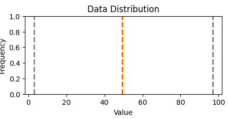
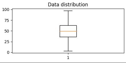
  • mean(simple average)
  • median(value in the middle)
  • mode(most common occurring value)

%matplotlib inline

from matplotlib import pyplot as plt

# Var to examine
var = df_students['Grade']

# Statistics
min_val = var.min()
max_val = var.max()
mean_val = var.mean()
med_val = var.median()
mod_val = var.mode()[0]

print('Minimum:{:.2f}Mean:{:.2f}Median:{:.2f}Mode:{:.2f}Maximum:{:.2f}'.format(min_val, mean_val, med_val, mod_val, max_val))

# Set figure
fig = plt.figure(figsize=(5,2))

# Add lines
plt.axvline(x=min_val, color = 'gray', linestyle='dashed', linewidth=2)
plt.axvline(x=max_val, color = 'cyan', linestyle='dashed', linewidth=2)
plt.axvline(x=med_val, color = 'red', linestyle='dashed', linewidth=2)
plt.axvline(x=mod_val, color = 'yellow', linestyle='dashed', linewidth=2)
plt.axvline(x=max_val, color = 'gray', linestyle='dashed', linewidth=2)

# Text
# Add titles and labels
plt.title('Data Distribution')
plt.xlabel('Value')
plt.ylabel('Frequency')

# Show
fig.show()

Result:
Minimum:3.00
Mean:49.18
Median:49.50
Mode:50.00
Maximum:97.00


Two quartiles of the data reside: ~ 36 and 63, ie. 0-36 and 63-100
Grades are between 36 and 63.

As a summary: distribution and plot box in the same figure

Another way to visualize the distribution of a variable is to use a box plot (box-and-whiskers plot)
var = df_students['Grade']
fig = plt.figure(figsize=(5,2))
plt.boxplot(var)
plt.title('Data distribution')

fig.show()

It is diferent from Histogram.
Show that 50% of dataresides - in 2 quartiles (between 36% abn 63%), the other 50% of data are between 0 - 36% and 63% -10%

Most common approach to have at a glance all is to build Histogram and Boxplot in the same figure.
# Create a function show_distribution
def show_distribution(var_data):
from matplotlib import pyplot as plt
min_val = var_data.min()
max_val = var_data.max()
mean_val = var_data.mean()
med_val = var_data.median()
mod_val = var_data.mode()[0]

fig, ax = plt.subplots(2, 1, figsize = (5,3))
# Plot histogram
ax[0].hist(var_data)
ax[0].set_ylabel('Frequency')

#Draw vertical lines
ax[0].axvline(x=min_val, color = 'gray', linestyle='dashed', linewidth = 2)
ax[0].axvline(x=mean_val, color = 'cyan', linestyle='dashed', linewidth = 2)
ax[0].axvline(x=med_val, color = 'red', linestyle='dashed', linewidth = 2)
ax[0].axvline(x=mod_val, color = 'yellow', linestyle='dashed', linewidth = 2)
ax[0].axvline(x=max_val, color = 'gray', linestyle='dashed', linewidth = 2)

#Plot the boxplot
ax[1].boxplot(var_data, vert=False)
ax[1].set_xlabel('Value')
fig.suptitle('Data Distribution')

fig.show()

col = df_students['Grade']
#Call function
show_distribution(col)

Result:
Minimum:3.00
Mean:49.18
Median:49.50
Mode:50.00
Maximum:97.00


Central tendencyare right in the middle of the data distribution, which is symmetric with values becoming progressively lower in both directions from the middle
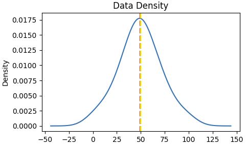
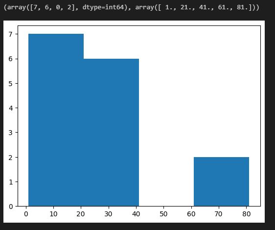
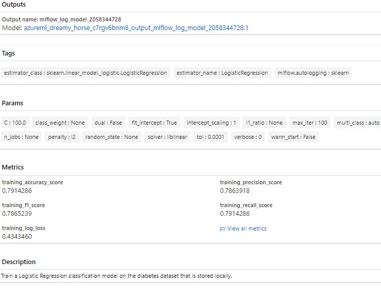
The Probability Density Functionis well implemented in pyplot

# Make sure you have scipy.
# How to install
# pip install scipy (run this in CS Code terminal

def show_density(var_data):
from matplotlib import pyplot as plt

fig = plt.figure(figsize=(10,4))

# Plot density
var_data.plot.density()

# Add titles and labels
plt.title('Data Density')

# Show the mean, median, and mode
plt.axvline(x=var_data.mean(), color = 'cyan', linestyle='dashed', linewidth = 2)
plt.axvline(x=var_data.median(), color = 'red', linestyle='dashed', linewidth = 2)
plt.axvline(x=var_data.mode()[0], color = 'yellow', linestyle='dashed', linewidth = 2)

# Show the figure
plt.show()

# Get the density of Grade
col = df_students['Grade']
show_density(col)


The density shows the characteristic "bell curve" of what statisticians call a normal distribution with the mean and mode at the center and symmetric tails.


References:
Exam DP-100: Designing and Implementing a Data Science Solution on Azure - Certifications | Microsoft Learn
Welcome to Python.org
pandas - Python Data Analysis Library (pydata.org)
Matplotlib — Visualization with Python0

Visual Studio code - Azure CLI basic

Study notes

Why Azure CLI
To train a model with Azure Machine Learning workspace, you can use:
  1. Designer in the Azure Machine Learning Studio
  2. Python SDK
  3. Azure CLI. To automate the training and retraining of models more effectively, the CLI is the preferred approach.
Open VS code and then a Power Shell. Run:
az --version
Result:
azure-cli 2.45.0
....
Extensions:
ml 2.14.0

You must have version 2.x for both.

if not run:
az upgrade
az extension remove -n azure-cli-ml
az extension remove -n ml
az extension add -n ml -y

Assume you are logged in (if not az login)
Check/ set active subscription.
az account show
# get the current default subscription using show
az account show --output table
# get the current default subscription using list
az account list --query "[?isDefault]"
# change the active subscription using the subscription ID
az account set --s "xxxxxxxx-xxxx-xxxx-xxxx-xxxxxxxxxxxx"

Create resource group
# It will be created in active subscription
az group create --name "GROUP_NAME"--location "eastus"
# Set it default
az configure --defaults group="GROUP_NAME"

Create workspace
# It will be created in active scubscription and default resource grop
az ml workspace create --name "WS_NAME"
#Set the default workspace
az configure --defaults workspace="WS_NAME"

Create compute instance
# It will be created in active subscription and default resourcegroup and default workspace
#--resource-group: Name of resource group. If you configured a default group with az configure --defaults group=<name>, you don't need to use this parameter.
#--workspace-name: Name of the Azure Machine Learning workspace. If you configured a default workspace with az configure --defaults workspace=<name>, you don't need to use this parameter.
#--name: Name of compute target. The name should be fewer than 24 characters and unique within an Azure region.
#--size: VM size to use for the compute instance. Learn more about supported VM series and sizes.
#--type: Type of compute target. To create a compute instance, use ComputeInstance
az ml compute create --name "INSTANCE_NAME" --size STANDARD_DS11_V2 --type ComputeInstance

Create compute cluster
# It will be created in active subscription and default resourcegroup and default workspace
#--type: To create a compute cluster, use AmlCompute.
#--min-instances: The minimum number of nodes used on the cluster. The default is 0 nodes.
#--max-instances: The maximum number of nodes. The default is 4.
az ml compute create --name "CLUSTER_NAME" --size STANDARD_DS11_V2 --max-instances 2 --type AmlCompute

Create dataset
Necessary two files:
data_local_path.yaml
$schema: https://azuremlschemas.azureedge.net/latest/data.schema.json
name: lab-data
version: 1
path: data
description: Dataset pointing to diabetes data stored as CSV on local computer. Data is uploaded to default datastore.
lab.data.csv

Run:
az ml data create -- file ./PATH_TO_YAML_FILE/data_local_path.yaml

When you create a dataset from a local path, the workspace will automatically upload the dataset to the default datastore. In this case, it will be uploaded to the storage account which was created when you created the workspace.
Once the dataset is created, a summary is shown in the prompt. You can also view the environment in the Azure ML Studio in the Environments tab.

List datastores
az ml datastore list

Find it in Azure UI
Storage (Under resource where is the Azure ML workspace)
  • Storage browser
  • Blob containers
  • azureml-blobstore.....
  • LocalUpload
Here are all about Azure ML including data related with the environment.

Create environment.
You expect to use a compute cluster in the future to retrain the model whenever needed. To train the model on either a compute instance or compute cluster, all necessary packages need to be installed on the compute to run the code. Instead of manually installing these packages every time you use a new compute, you can list them in an environment.
Every Azure Machine Learning workspace will by default have a list of curated environments when you create the workspace. Curated environments include common machine learning packages to train a model.
Necessary two files (in the same folder for this example):

basic-env-ml.yml
name: basic-env-ml
channels:
- conda-forge
dependencies:
- python=3.8
- pip
- pip:
- numpy
- pandas
- scikit-learn
- matplotlib
- azureml-mlflow

basic-env.yml

$schema: https://azuremlschemas.azureedge.net/latest/environment.schema.json
name: basic-env-scikit
version: 1
image: mcr.microsoft.com/azureml/openmpi3.1.2-ubuntu18.04
conda_file: file:conda-envs/basic-env-ml.yml

Run
az ml environment create --file ./PATH_TO_YAML_FILE/basic-env.yml

Stop instance:
az ml compute stop --name "INSTANCE_NAME"

List resources groups
az group list --output table

Delete resource group
az group delete --name GROUP_NAME

Delete workspace
az ml workspace delete


References:
How to manage Azure resource groups – Azure CLI | Microsoft Learn
Manage workspace assets with CLI (v2) - Training | Microsoft Learn

Purebred Dog Breeds

Docker containers basic

Study notes

Container
Runnable instance of a container image isolated from other containers.

Container image
Contains the container filesystem and everything necessary to run the application including dependencies, environment variables, default command to run when start the container and other metadata.
It is a read-only template with instructions for creating a docker container.
An image can be based on other images, ie. it is based on unbutu but contains Apache.
To create an image, it is necessary the Dockerfile(contains steps to create the image and run it)

Containerize an application
Set the getting-started app.

1. Get the app
Clone the getting-started repository using the following command
git clone https://github.com/docker/getting-started.git

In VS code you have


2. Build the app’s container image
Create Dockerfile in /app folder.
# syntax=docker/dockerfile:1
FROM node:18-alpine
WORKDIR /app
COPY . .
RUN yarn install --production
CMD ["node", "src/index.js"]
EXPOSE 3000

In terminal (in /app folder, run:
docker build -t getting-started .

Build command uses the Dockerfile to build a new container image.
Docker downloaded a lot of “layers”: you want to start from the node:18-alpine image but, since you didn’t have that on your machine Docker will download it.
Then yarn install your application’s dependencies.
The CMD directive specifies the default command to run when starting a container from this image.
Expose - what port will be used to load app.
-t flag tags your image. Think of this simply as a human-readable name for the final image.
Since you named the image getting-started, you can refer to that image when you run a container.

3. Start an app container
docker run -dp 3000:3000 getting-started

You can stop and remove the container from terminal or VS code.


Share the application
Upload image to docker hub repository

1. Go to
Docker Hub (sign in)
Create a repository:
name: getting-started
visibility: public

In VS code terminal, /app folder
2. Login:
docker login -u YOUR-USER-NAME .

3. Use the docker tag command to give the getting-started image a new name. Be sure to swap out YOUR-USER-NAME with your Docker ID
docker tag getting-started YOUR-USER-NAME/getting-started

4. Push (Upload) image to Docker hub (in repository created
docker push YOUR-USER-NAME/getting-started

5. Check, run image on a new instance
Test in Docker playground
Load and sign in: Play with Docker (play-with-docker.com)

Add New instance
Run in terminal:
docker run -dp 3000:3000 YOUR-USER-NAME/getting-started


Click on 3000 ports. Brows should open and app will run.

Close session

Persist the DB
Each container also gets its own “scratch space” to create/update/remove files. Any changes won’t be seen in another container, even if they are using the same image

In terminal (your folder root, not in app - not relevant anyway here)

docker run -d ubuntu bash -c "shuf -i 1-10000 -n 1 -o /data.txt && tail -f /dev/null"

An image will be created from ubuntu and execute:
stuff -i 1-10000 -n 1 -o /data.txt
Generate numbers between 1 and 10000, take maximum ONE (1) and write in /data.txt file. Output discarded.

See data.txt in Docker desktop, VS code and in terminal:
docker exec <container-id> cat /data.txt
Remove container:
docker stop <container-id>
docker rm<container-id>

Create a new container (list file when done)
# -i means interactive
# -t mean stty
# -itmeans start a container and go stright into container.
# -d means start the container and then detach from it
docker run -it ubuntu ls /
No data.txt file

Persist the todo data
By default, the todo app stores its data in a SQLite database at /etc/todos/todo.db in the container’s filesystem
With the database being a single file, if we can persist that file on the host and make it available to the next container, it should be able to pick up where the last one left off.
By creating a volume and attaching (often called “mounting”) it to the directory the data is stored in, we can persist the data.

Share a point in a volume to the container.

1. Create volume
docker volume create todo-db

2. Start the todo app container, but add the --mountoption to specify a volume mount.
We will give the volume a name, and mount it to /etc/todos in the container, which will capture all files created at the path.
docker run -dp 3000:3000 --mount type=volume,src=todo-db,target=/etc/todos getting-started

Load
https://localhost:3000

Add items.
Stop, remove container.
Start again with the same command.
docker run -dp 3000:3000 --mount type=volume,src=todo-db,target=/etc/todos getting-started

Load
https://localhost:3000
Items are there even container was removed.

Data is stored here:
docker volume inspect todo-db
Result:
[
{
"CreatedAt": "2023-01-29T02:24:06Z",
"Driver": "local",
"Labels": {},
"Mountpoint": "/var/lib/docker/volumes/todo-db/_data",
"Name": "todo-db",
"Options": {},
"Scope": "local"
}
]


Bind mounts
Share a directory from the host’s filesystem into the container.
When working on an application, you can use a bind mount to mount source code into the container.
The container sees the changes you make to the code immediately, as soon as you save a file. This means that you can run processes in the container that watch for filesystem changes and respond to them.
In this chapter, we’ll see how we can use bind mounts and a tool called nodemonto watch for file changes, and then restart the application automatically.

.Named volumesBind mounts
Host locationDocker choosesYou decide
Mount example (using --mount)type=volume,src=my-volume,target=/usr/local/datatype=bind,src=/path/to/data,target=/usr/local/data
Populates new volume with container contentsYesNo
Supports Volume DriversYesNo

Trying out bind mounts

VS code terminal - /app folder
Create & start container from ubuntu image, mount current host file system (the /app folder) into corresponding folder in /src subfolder ... app/src
getting-started/app => /src

root@48b82c33f7ea:/# ls
bin boot dev etc home lib lib32 lib64 libx32 media mnt opt proc root run sbin src srv sys tmp usr var
root@48b82c33f7ea:/# cd sr
src/ srv/
root@48b82c33f7ea:/# cd src
root@48b82c33f7ea:/src# ls
Dockerfile package.json spec src yarn.lock
root@48b82c33f7ea:/src# touch myfile.txt
root@48b82c33f7ea:/src# ls
Dockerfile myfile.txt package.json spec src yarn.lock

# myfile.txt exist on local filesystem
# delete it from local file system (host)

root@48b82c33f7ea:/src# ls
Dockerfile package.json spec src yarn.lock
# was deleted from docker container
root@48b82c33f7ea:/src#
exit
PS C:UsersUSERDocumentslocaldevDocker_learnapp>

Run your app in a development container
Make sure you have a fresh copy of getting-started in folder

Co to /app folder
In PowerShellrun
docker run -dp 3000:3000 `
-w /app --mount type=bind,src="$(pwd)",target=/app `
node:18-alpine `
sh -c "yarn install && yarn run dev"

  • -dp 3000:3000 - same as before. Run in detached (background) mode and create a port mapping
  • -w /app - sets the “working directory” or the current directory that the command will run from
  • --mount type=bind,src="$(pwd)",target=/app - bind mount the current directory from the host into the /app directory in the container
  • node:18-alpine - the image to use. Note that this is the base image for our app from the Dockerfile
  • sh -c "yarn install && yarn run dev" - the command. We’re starting a shell usingsh (alpine doesn’t have bash) and running yarn installto install packages and then running yarn run devto start the development server. If we look in the package.json, we’ll see that the dev script startsnodemon.

You can watch the logs using docker logs

...app> docker logs -f 90dfac47e8b2
yarn install v1.22.19
[1/4] Resolving packages...
[2/4] Fetching packages...
[3/4] Linking dependencies...
[4/4] Building fresh packages...
Done in 59.82s.
yarn run v1.22.19
$ nodemon src/index.js
[nodemon] 2.0.20
[nodemon] to restart at any time, enter `rs`
[nodemon] watching path(s): *.*
[nodemon] watching extensions: js,mjs,json
[nodemon] starting `node src/index.js`

Using sqlite database at /etc/todos/todo.db
Listening on port 3000

nodemonis running and watching any change.

When you’re done watching the logs, exit out by hitting Ctrl+C.

Feel free to make any other changes you’d like to make. Each time you make a change and save a file, the nodemon process restarts the app inside the container automatically. When you’re done, stop the container and build your new image using:
docker build -t getting-started .

Multi container apps
Networking - Allow one container to talk to another.
If twocontainers are on the same network, they can talk to each other. If they aren’t, they can’t.

# Create network
docker network create todo-app

# Start a MySQL container and attach it to the network
docker run -d `
--network todo-app --network-alias mysql `
-v todo-mysql-data:/var/lib/mysql `
-e MYSQL_ROOT_PASSWORD=secret`
-e MYSQL_DATABASE=todos `
mysql:8.0

Connect to MySQL
docker exec -it a40b6d2feb91 mysql -u root -p
(pass ...see above)

Connect to MySQL
If we run another container on the same network, how do we find the container (remember each container has its own IP address)?
To figure it out, we’re going to make use of the nicolaka/netshoot container, which ships with a lot of tools that are useful for troubleshooting or debugging networking issues.

1. Start a new container using the nicolaka/netshoot image. Make sure to connect it to the same network.
docker run -it --network todo-app nicolaka/netshoot


# Mysql is the network alias used when container was created
dig mysql

<<>> DiG 9.18.8 <<>> mysql
;; global options: +cmd
;; Got answer:
;; ->>HEADER<<- opcode: QUERY, status: NOERROR, id: 63746
;; flags: qr rd ra; QUERY: 1, ANSWER: 1, AUTHORITY: 0, ADDITIONAL: 0

;; QUESTION SECTION:
;mysql. IN A

;; ANSWER SECTION:
mysql. 600 IN A 172.18.0.2

;; Query time: 10 msec
;; SERVER: 127.0.0.11#53(127.0.0.11) (UDP)
;; WHEN: Sun Jan 29 04:13:04 UTC 2023
;; MSG SIZE rcvd: 44


Docker was able to resolve it to the IP address of the container that had that network alias (remember the --network-alias flag we used earlier?).

Run your app with MySQL

The todo app supports the setting of a few environment variables to specify MySQL connection settings. They are:
  • MYSQL_HOST - the hostname for the running MySQL server
  • MYSQL_USER - the username to use for the connection
  • MYSQL_PASSWORD - the password to use for the connection
  • MYSQL_DB - the database to use once connected
Secure mechanism is to use the secret support provided by your container orchestration framework
In most cases, these secrets are mounted as files in the running container. You’ll see many apps (including the MySQL image and the todo app) also support env vars with a _FILE suffix to point to a file containing the variable.

As an example, setting the MYSQL_PASSWORD_FILE var will cause the app to use the contents of the referenced file as the connection password. Docker doesn’t do anything to support these env vars. Your app will need to know to look for the variable and get the file contents.

1. Note: for MySQL versions 8.0 and higher, make sure to include the following commands in mysql
mysql>ALTER USER 'root' IDENTIFIDE WITH mysql_natve_password BY 'secret'
mysql>flush privileges

2. We’ll specify each of the environment variables above, as well as connect the container to our app network.
docker run -dp 3000:3000 `
-w /app -v "$(pwd):/app" `
--network todo-app `
-e MYSQL_HOST=mysql `
-e MYSQL_USER=root `
-e MYSQL_PASSWORD=secret `
-e MYSQL_DB=todos `
node:18-alpine `
sh -c "yarn install && yarn run dev"

3. If we look at the logs for the container
docker logs -f <container-id>
we should see a message indicating it’s using the mysql database

4.Open the app in your browser and add a few items to your todo list.

5. Connect to the mysql database and prove that the items are being written to the database. Remember, the password is secret.
docker exec -it <mysql-container-id> mysql -p todos

Use Docker Compose
Docker Compose is a tool that was developed to help define and share multi-container applications.

1. At the root of the app project, create a file named
docker-compose.yml
# and start with
services:

2. In the compose file, we’ll start off by defining the list of services (or containers) we want to run as part of our application.
First is the app container
It was created with:
docker run -dp 3000:3000
-w /app -v "$(pwd):/app"
--network todo-app
-e MYSQL_HOST=mysql
-e MYSQL_USER=root
-e MYSQL_PASSWORD=secret
-e MYSQL_DB=todos
node:18-alpine
sh -c "yarn install && yarn run dev"

Then was created:
docker run -d
--network todo-app --network-alias mysql
-v todo-mysql-data:/var/lib/mysql
-e MYSQL_ROOT_PASSWORD=secret
-e MYSQL_DATABASE=todos
mysql:8.0

So, we have
services:
app:
image: node:18-alpine
command: sh -c "yarn install && yarn run dev"
ports:
- 3000:3000
working_dir: /app
# Above coming from -w /app
volumes:
- ./:/app
# Above coming from -v "$(pwd):/app"
environment:
MYSQL_HOST: mysql
MYSQL_USER: root
MYSQL_PASSWORD: secret
MYSQL_DB: todos
# Above coming from:
#-e MYSQL_HOST=mysql
#-e MYSQL_USER=root
#-e MYSQL_PASSWORD=secret
#-e MYSQL_DB=todos

mysql:
image: mysql:8.0
volumes:
- todo-mysql-data:/var/lib/mysql
environment:
MYSQL_ROOT_PASSWORD: secret
MYSQL_DATABASE: todos
#Below have NO IDEEA Yet!!!
volumes:
todo-mysql-data:

Run the application stack
You will get 2 running containers.


Open:
localhost:3000
App must work

Check Mysql:
docker exec -it 36e1e8b918b2 mysql -p todos
#Then in mysql you will see what just entered in app
use todos';
select * from todo_items;
+--------------------------------------+------+-----------+
| id | name | completed |
+--------------------------------------+------+-----------+
| 972352e4-aa42-412a-bea2-e44a5419451b | 11 | 0 |
| 36b97346-2761-4b4e-a835-24a9b7767cec | 22 | 0 |
| bd05ef47-1033-468a-888e-65c79ed5ae64 | 33 | 0 |
+--------------------------------------+------+-----------+
3 rows in set (0.00 sec)

Removing Volumes
By default, named volumes in your compose file are NOT removed when running docker compose down. If you want to remove the volumes, you will need to add the --volumes flag.
The Docker Dashboard does not remove volumes when you delete the app stack.

Image-building best practices

Security scan

docker scan mysql

Tested 3 dependencies for known vulnerabilities, no vulnerable paths found.
For more free scans that keep your images secure, sign up to Snyk at https://dockr.ly/3ePqVcp

Image layering
Using the docker image history command, you can see the command that was used to create each layer within an image.
docker image history mysql
#or
docker image --no-trunc history mysql

Image layering

# Shows all layers of an image (how was built)
# Use --no-trunc to see all details
docker image history

Layer caching

Each command in the Dockerfile becomes a new layer in the image.
You might remember that when we made a change to the image, the yarn dependencies had to be reinstalled
To fix this, we need to restructure our Dockerfile to help support the caching of the dependencies. For Node-based applications, those dependencies are defined in the package.json file. So, what if we copied only that file in first, install the dependencies, and then copy in everything else? Then, we only recreate the yarn dependencies if there was a change to the package.json.

From this (bad)

# syntax=docker/dockerfile:1
FROM node:18-alpine
WORKDIR /app
COPY . .
RUN yarn install --production
CMD ["node", "src/index.js"]

To this:

# syntax=docker/dockerfile:1
FROM node:18-alpine
WORKDIR /app
COPY package.json yarn.lock ./
RUN yarn install --production
COPY . .
CMD ["node", "src/index.js"]

Create a file named .dockerignore in the same folder as the Dockerfile with the following contents.
Example:
# comment
*/temp*
*/*/temp*
temp?

Rebuilding images -> system use cache

Multi-stage builds

Incredibly powerful tool to help use multiple stages to create an image.

  • Separate build-time dependencies from runtime dependencies
  • Reduce overall image size by shipping only what your app needs to run
React example

When building React applications, we need a Node environment to compile the JS code (typically JSX), SASS stylesheets, and more into static HTML, JS, and CSS.
If we aren’t doing server-side rendering, we don’t even need a Node environment for our production build. So, ship the static resources in a static nginx container.

# syntax=docker/dockerfile:1
FROM node:18 AS build
WORKDIR /app
COPY package* yarn.lock ./
RUN yarn install
COPY public ./public
COPY src ./src
RUN yarn run build

FROM nginx:alpine
COPY --from=build /app/build /usr/share/nginx/html


References:
Overview | Docker Documentation
Reference documentation | Docker Documentation
Vulnerability scanning for Docker local images | Docker Documentation
nodemon - npm (npmjs.com)

Visual Studio code - Azure CLI - ML manage jobs

Study notes

Setup VS code for ML Jobs:
Visual Studio code - Azure CLI basic (cristinabrata.com)
Summary
VS code has set the default Azure Workspace and Environment
  1. Script
  2. Environment
  3. Compute
Create environment.
You expect to use a compute cluster in the future to retrain the model whenever needed. To train the model on either a compute instance or compute cluster, all necessary packages need to be installed on the compute to run the code. Instead of manually installing these packages every time you use a new compute, you can list them in an environment.
Every Azure Machine Learning workspace will by default have a list of curated environments when you create the workspace. Curated environments include common machine learning packages to train a model.

Necessary two files a .py and a .yml (in the same folder for this example):

basic-env-ml.yml
name: basic-env-ml
channels:
- conda-forge
dependencies:
- python=3.8
- pip
- pip:
- numpy
- pandas
- scikit-learn
- matplotlib
- azureml-mlflow
basic-env.yml


$schema: https://azuremlschemas.azureedge.net/latest/environment.schema.json
name: basic-env-scikit
version: 1
image: mcr.microsoft.com/azureml/openmpi3.1.2-ubuntu18.04
conda_file: file:conda-envs/basic-env-ml.yml
Run
az ml environment create --file ./PATH_TO_YAML_FILE/basic-env.yml


Train the model (Create Azure ML job)
Theer are one .yaml and one .py files

main.py
The code that generate the experiment / job.
All in here will be exceuted in Azure on the instance/cluster set in data_job.yaml
Immediately job is created, it starts.

# Import libraries
import mlflow
import argparse

import pandas as pd
from sklearn.model_selection import train_test_split
from sklearn.linear_model import LogisticRegression

# define functions
def main(args):
# enable auto logging
mlflow.autolog()
# read data
df = pd.read_csv('diabetes.csv')
# process data
X_train, X_test, y_train, y_test = process_data(df)

# train model
model = train_model(args.reg_rate, X_train, X_test, y_train, y_test)
def process_data(df):
# split dataframe into X and y
X, y = df[['Pregnancies','PlasmaGlucose','DiastolicBloodPressure','TricepsThickness','SerumInsulin','BMI','DiabetesPedigree','Age']].values, df['Diabetic'].values

# train/test split
X_train, X_test, y_train, y_test = train_test_split(X, y, test_size=0.30, random_state=0)

# return splits and encoder
return X_train, X_test, y_train, y_test

def train_model(reg_rate, X_train, X_test, y_train, y_test):
# train model
model = LogisticRegression(C=1/reg_rate, solver="liblinear").fit(X_train, y_train)

# return model
return model

def parse_args():
# setup arg parser
parser = argparse.ArgumentParser()

# add arguments
parser.add_argument("--reg-rate", dest="reg_rate", type=float, default=0.01)

# parse args
args = parser.parse_args()

# return args
return args

# run script
if __name__ == "__main__":
# add space in logs
print(" ")
print("*" * 60)

# parse args
args = parse_args()

# run main function
main(args)

# add space in logs
print("*" * 60)
print(" ")

data_job.yml
This is the file run in CLI
$schema: https://azuremlschemas.azureedge.net/latest/commandJob.schema.json
# folder where is main_py
code: src
command: >-
python main.py
--diabetes-csv ${{inputs.diabetes}}
inputs:
diabetes:
path: azureml:diabetes-data:1
mode: ro_mount
# it is already creatde
environment: azureml:basic-env-scikit@latest
# It is created and running (if stoped - job will be set in queue
compute: azureml:COMPUTE_INSTANCE_OR_CLUSTER
experiment_name: diabetes-data-example
description: Train a classification model on diabetes data using a registered dataset as input.

Run
# When you include the parameter --web, a web page will open after the job is submitted so you can monitor the experiment run in the Azure Machine Learning Studio.
az ml job create --file ./PATH_TO_YAML_FILE/basic-job.yml --web

We can se job in Azure ML Studio.


Add dataset as input to job

Important is to retrain the model and from time to time use a new dataset to keep it up to date and make it better.
To easily change the input dataset every time you want to retrain the model, you want to create an input argument for the data.
Replace locally stored CSV (from the training script) with an YAML file.
  1. In the script
    You define the input arguments using the argparse module. You specify the argument's name, type and optionally a default value.
  2. In the YAML file:
    You specify the data input, which will mount (default option) or download data to the local file system. You can refer to a public URI or a registered dataset in the Azure Machine Learning workspace.

Train a new model:
There are one .yml and one .py files

main.py
The code that generate the experiment / job.
All in here will be exceuted in Azure on the instance/cluster set in data_job.yaml
Immediately job is created, it starts.

# Import libraries
import mlflow
import argparse
import glob

import pandas as pd
from sklearn.model_selection import train_test_split
from sklearn.linear_model import LogisticRegression

# IT WAS
# read data
# df = pd.read_csv('diabetes.csv')

# define functions
def main(args):
# enable auto logging
mlflow.autolog()

# read data
data_path = args.diabetes_csv
all_files = glob.glob(data_path + "/*.csv")
df = pd.concat((pd.read_csv(f) for f in all_files), sort=False)

# process data
X_train, X_test, y_train, y_test = process_data(df)

# train model
model = train_model(args.reg_rate, X_train, X_test, y_train, y_test)

def process_data(df):
# split dataframe into X and y
X, y = df[['Pregnancies','PlasmaGlucose','DiastolicBloodPressure','TricepsThickness','SerumInsulin','BMI','DiabetesPedigree','Age']].values, df['Diabetic'].values

# train/test split
X_train, X_test, y_train, y_test = train_test_split(X, y, test_size=0.30, random_state=0)

# return splits and encoder
return X_train, X_test, y_train, y_test

def train_model(reg_rate, X_train, X_test, y_train, y_test):
# train model
model = LogisticRegression(C=1/reg_rate, solver="liblinear").fit(X_train, y_train)

# return model
return model

def parse_args():
# setup arg parser
parser = argparse.ArgumentParser()

# add arguments
parser.add_argument("--diabetes-csv", dest='diabetes_csv', type=str)
parser.add_argument("--reg-rate", dest='reg_rate', type=float, default=0.01)

# parse args
args = parser.parse_args()

# return args
return args

# run script
if __name__ == "__main__":
# add space in logs
print(" ")
print("*" * 60)

# parse args
args = parse_args()

# run main function
main(args)

# add space in logs
print("*" * 60)
print(" ")

data_job.yml
This is the file run in CLI

$schema: https://azuremlschemas.azureedge.net/latest/commandJob.schema.json
# folder where is main_py
code: src
command: >-
python main.py
# bellow is new
--diabetes-csv ${{inputs.diabetes}}
inputs:
diabetes:
path: azureml:diabetes-data:1
mode: ro_mount
# above is new
# it is already creatde
environment: azureml:basic-env-scikit@latest
# It is created and running (if stoped - job will be set in queue
compute: azureml:COMPUTE_INSTANCE_OR_CLUSTER
experiment_name: diabetes-data-example
description: Train a classification model on diabetes data using a registered dataset as input.

Run
# When you include the parameter --web, a web page will open after the job is submitted so you can monitor the experiment run in the Azure Machine Learning Studio.
az ml job create --file ./PATH_TO_YAML_FILE/data-job.yml

Result from Azure ML Studio
Run a Job using hyperparameter (tune job)
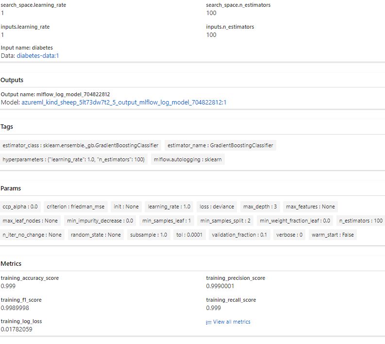
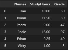
Perform hyperparameter tuning with the Azure Machine Learning workspace by submitting a sweep job.
Use a sweep job to configure and submit a hyperparameter tuning job via the CLI (v2).

Hyperparametertuning allows to train multiple models, using the same algorithm and training data but different hyperparameter values.
For each iteration, the performance metrics need to be tracked to evaluate which configuration resulted in the best model.

Target - Instance cluster.

If you have note run:
az ml compute create --name "CLUSTER_NAME" --size STANDARD_DS11_V2 --max-instance 2 --type AmlCompute

There are two files; a .py and a .yml

main.py
Contains the python script that train the model (write and test in Jupyter note and pack it here)
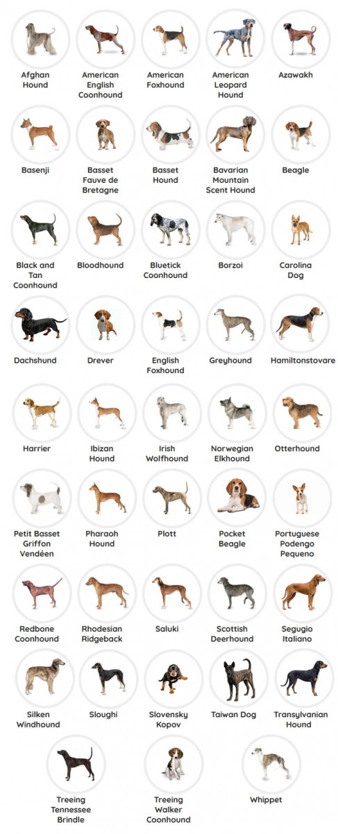
import mlflow
import argparse
import glob

import pandas as pd
from sklearn.model_selection import train_test_split
from sklearn.ensemble import GradientBoostingClassifier

# define functions
def main(args):
# enable auto logging
mlflow.autolog()
params = {
"learning_rate": args.learning_rate,
"n_estimators": args.n_estimators,
}

# read data
data_path = args.diabetes_csv
all_files = glob.glob(data_path + "/*.csv")
df = pd.concat((pd.read_csv(f) for f in all_files), sort=False)
# process data
X_train, X_test, y_train, y_test = process_data(df)

# train model
model = train_model(params, X_train, X_test, y_train, y_test)
def process_data(df):
# split dataframe into X and y
X, y = df[['Pregnancies','PlasmaGlucose','DiastolicBloodPressure','TricepsThickness','SerumInsulin','BMI','DiabetesPedigree','Age']].values, df['Diabetic'].values

# train/test split
X_train, X_test, y_train, y_test = train_test_split(X, y, test_size=0.30, random_state=0)

# return splits and encoder
return X_train, X_test, y_train, y_test

def train_model(params, X_train, X_test, y_train, y_test):
# train model
model = GradientBoostingClassifier(**params)
model = model.fit(X_train, y_train)

# return model
return model

def parse_args():
# setup arg parser
parser = argparse.ArgumentParser()

# add arguments
parser.add_argument("--diabetes-csv", type=str)
parser.add_argument("--learning-rate", dest='learning_rate', type=float, default=0.1)
parser.add_argument("--n-estimators", dest='n_estimators', type=int, default=100)

# parse args
args = parser.parse_args()

# return args
return args

# run script
if __name__ == "__main__":
# add space in logs
print(" ")
print("*" * 60)

# parse args
args = parse_args()

# run main function
main(args)

# add space in logs
print("*" * 60)
print(" ")

There are two hyperparameter values:
  • Learning rate:
    with search space [0.01, 0.1, 1.0]
  • N estimators:
    with search space [10, 100]
sweep-job.yml
File to run - creates experiemnt.

$schema: https://azuremlschemas.azureedge.net/latest/sweepJob.schema.json
type: sweep
sampling_algorithm: grid
trial:
code: src
command: >-
python main.py
--diabetes-csv ${{inputs.diabetes}}
--learning-rate ${{search_space.learning_rate}}
--n-estimators ${{search_space.n_estimators}}
environment: azureml:basic-env-scikit@latest
inputs:
diabetes:
path: azureml:diabetes-data:1
mode: ro_mount
compute: azureml:CLUSTER_NAME
search_space:
learning_rate:
type: choice
values: [0.01, 0.1, 1.0]
n_estimators:
type: choice
values: [10, 100]
objective:
primary_metric: training_roc_auc_score
goal: maximize
limits:
max_total_trials: 6
max_concurrent_trials: 3
timeout: 3600
experiment_name: diabetes-sweep-example
description: Run a hyperparameter sweep job for classification on diabetes dataset.

Parameters:
  • type:
    The job type, which in this case is sweep_job.
  • algorithm:
    The sampling method used to choose values from the search space. Can be bayesian, grid, or random.
  • search_space:
    The set of values tried during hyperparameter tuning. For each hyperparameter, you can configure the search space type (choice) and values (0.01, 0.1, 1.0).
  • objective:
    The name of the logged metric that is used to decide which model is best (primary_metric). And whether that metric is best when maximized or minimized (goal).
  • max_total_trials:
    A hard stop for how many models to train in total.
  • max_concurrent_trials:
    When you use a compute cluster, you can train models in parallel. The number of maximum concurrent trials can't be higher than the number of nodes provisioned for the compute cluster.
Run to submit job:
az ml job create --file ./PATH_TO_JOB_FILE/sweep-job.yml

In Azure ML Studio
Best trial results:


References:
Train models in Azure Machine Learning with the CLI (v2) - Training | Microsoft Learn
Visual Studio code - Azure CLI basic (cristinabrata.com)
Train ML models - Azure Machine Learning | Microsoft Learn
az ml job | Microsoft Learn
azureml-examples/cli at main · Azure/azureml-examples (github.com)

Non-Shedding Dog

Docker in Visual Studio Code

Study notes

What for Docker here; statistics and Azure ML?

When create experiments no everything is going well and you need to debug.
If it is about a deep learning, convulsive neural networks or just an experiment that require AKS clusters then the recommended option is to run your buggy experiment in a container on Docker and then send back to cloud into AKS cluster.

Good news is that Visual Studio code make our life easier.

Initial steps:
The extension can scaffold Docker files for most popular development languages (C#, Node.js, Python, Ruby, Go, and Java) and customizes the generated Docker files accordingly.

The app has to be set into set into the folder
Docker/Node.js steps:
Open a terminal (command prompt in VS code) and install express (Node.js)
>npx express-generator
>npm install

Open Command Palette and

  • Generate Docker file
Command Palette and type:
>Docker: Add Docker Files to Workspace command
If image selected is node.js then:
- before doing this install node, yo can do it in terminal (VS code)
- you may get an error: "No package .json found on workspace"

Open a terminal and run:
>npm init
Now I assume the "Docker: Add Docker Files to Workspace" command works.


Main resources:
https://code.visualstudio.com/docs/containers/overview
https://docs.docker.com/desktop/

Herding Dogs

Docker from create container to deployment in Azure

Study Notes

Mounting
Volumes
Docker manage the mount points and data.
Use it if want to store your container’s data on a remote host and not locally.

Bind (need it here)
Use it if you want to save your data locally on the host itself or want to share data from your Docker host to the Docker container especially, configuration files, source code, etc.

#Works in PowerShell only , command prompt have not pwd
docker run -it --mount type=bind,src="$(pwd)",target=/src ubuntu bash

tmpfs (not relevant here)
Best for sensitive data or information, you do not want the data to be saved on the host machine or docker container (store secret keys for an example)

Data does not persist in container (run)

Create container, create file and write a random number to it.
docker run -d ubuntu bash -c "shuf -i 1-10000 -n 1 -o /data.txt && tail -f /dev/null"
docker ps
Result:
CONTAINER ID IMAGE COMMAND CREATED STATUS PORTS NAMES
834744ade459 ubuntu "bash -c 'shuf -i 1-…" 3 minutes ago Up 3 minutes silly_clarke

Read data.txt content
docker exec 834744ade459 cat /data.txt
# or
docker run -it ubuntu cat /data.txt
Result:
8072

Delete container and create from the same image a new one
docker rm 834744ade459
docker run -it ubuntu ls
# or
docker exec 834744ade459ls

Result:
bin dev home lib32 libx32 mnt proc run srv tmp var
boot etc lib lib64 media opt root sbin sys usr
No data.txt

Data (and code) persists in container image

git clone https://github.com/docker/getting-started.git
cd app

Create Docker file
# syntax=docker/dockerfile:1
FROM node:18-alpine
WORKDIR /app
COPY . .
RUN yarn install --production
CMD ["node", "src/index.js"]
EXPOSE 3000

Create image getting-started
docker build -t getting-started .

Edit and change something in (line #56 for example) in /app/src/static/js/ap.js
Create new image
docker build -t getting-started1 .

Create and run container from getting-started
docker run -dp 3000:3000 getting-started
Open http:://localhost:3000
See intial code

Create and run container from getting-started1
docker run -dp 3001:3000 getting-started
Open http:://localhost:3001
See changed code

  • Keep versions of code in container image.
  • Keep data in container volumes, see next.

Persist data between runs

Use the same git image like above and create a container.

git clone https://github.com/docker/getting-started.git
cd app
Create Docker file
# syntax=docker/dockerfile:1
FROM node:18-alpine
WORKDIR /app
COPY . .
RUN yarn install --production
CMD ["node", "src/index.js"]
EXPOSE 3000
Create image getting-started
docker build -t getting-started .

Using SQLLite
By default, the todo app stores its data in a SQLite database at /etc/todos/todo.db in the container’s filesystem
With the database being a single file, if we can persist that file on the host and make it available to the next container, it should be able to pick up where the last one left off.
By creating a volume and attaching (mounting) it to the directory the data is stored in, we can persist the data.
As our container writes to the todo.db file, it will be persisted to the host in the volume.

docker volume create persistent-data-db
docker run -dp 3000:3000 --mount type=volume,src=persistent-data-db,target=/etc/todos getting-started

Load:
http://localhost:3000
Add some items
Stop & delete getting-started container

Run it again
docker run -dp 3000:3000 --mount type=volume,src=persistent-data-db,target=/etc/todos getting-started

All entered before is still there.


MySQL volume and Compose
Compose makes it getting interesting

Create MySQL volume

Multiline command in PowerShell (for Linux replace ` with backslash)
docker run -d `
--network todo-app --network-alias mysql `
-v todo-mysql-data:/var/lib/mysql `
-e MYSQL_ROOT_PASSWORD=secret `
-e MYSQL_DATABASE=todos `
mysql:8.0

Connect to database:
docker exec -it 7f5291ecd67e mysql -u root -p
# or interactive
docker exec -it 7f5291ecd67e bash
#mysql -u root -p
..
..
mysql> show databases;
+--------------------+
| Database |
+--------------------+
| information_schema |
| mysql |
| performance_schema |
| sys |
| tods |
+--------------------+
5 rows in set (0.00 sec)
mysql> quit

Use compose
Allows to create multiple containers and the environment. Manage all from a file.
You may say infrastructure as code at small scale in this case.

Same git source like above.
in /app create a file docker-compose.yml
When run, this will create 3
services:
app:
image: node:18-alpine
command: sh -c "yarn install && yarn run dev"
ports:
- 3000:3000
working_dir: /app
volumes:
- ./:/app
environment:
MYSQL_HOST: mysql
MYSQL_USER: root
MYSQL_PASSWORD: secret
MYSQL_DB: todos

mysql:
image: mysql:8.0
volumes:
- todo-mysql-data:/var/lib/mysql
environment:
MYSQL_ROOT_PASSWORD: secret
MYSQL_DATABASE: todos

volumes:
todo-mysql-data:

Run
docker compose up -d

All you change in codes source locally reflect into app container immediately (on reload)

To see database / tables:
docker exec -it 86230b97c184 bash
bash-4.4# mysql -u root -p
#Enter password:
Welcome to the MySQL monitor. Commands end with ; or g.
Your MySQL connection id is 12
...
mysql> show databases;
+--------------------+
| Database |
+--------------------+
| information_schema |
| mysql |
| performance_schema |
| sys |
| todos |
+--------------------+
5 rows in set (0.00 sec)

mysql> use todos;
Database changed
mysql> show tables;
+-----------------+
| Tables_in_todos |
+-----------------+
| todo_items |
+-----------------+
1 row in set (0.01 sec)

mysql> select * from todo_items;
+--------------------------------------+------+-----------+
| id | name | completed |
+--------------------------------------+------+-----------+
| 68e9fc83-66b8-406e-b404-8899d5570c36 | sdfg | 0 |
| 1c441ab9-4d8d-45a8-865e-f2b49494e6cc | sdfg | 0 |
+--------------------------------------+------+-----------+
2 rows in set (0.00 sec)

mysql> delete from todo_items;
Query OK, 2 rows affected (0.01 sec)

mysql> select * from todo_items;
Empty set (0.01 sec)

mysql>quit


Shut it down:
docker compose down

Containers are stopped and deleted
Images stay.
Volume with data stay

Create & start images.
docker composeup -d
All is back - no database lost

CI/CD pipe

Terms

1. venv
Creation of virtual environments — Python 3.11.1 documentation
The venv module supports creating lightweight “virtual environments”, each with their own independent set of Python packages installed in theirsite directories. A virtual environment is created on top of an existing Python installation, known as the virtual environment’s “base” Python, and may optionally be isolated from the packages in the base environment, so only those explicitly installed in the virtual environment are available.
When used from within a virtual environment, common installation tools such aspip will install Python packages into a virtual environment without needing to be told to do so explicitly.

2. PEP 405
Python Virtual Environments
This PEP proposes to add to Python a mechanism for lightweight “virtual environments” with their own site directories, optionally isolated from system site directories. Each virtual environment has its own Python binary (allowing creation of environments with various Python versions) and can have its own independent set of installed Python packages in its site directories but shares the standard library with the base installed Python.

Create a flask web server container
python3 -m venv .venv
# on windows
.venvScriptsace
python3 -m flask run

Tag it and check
docker build --tag python-docker .
curl localhost:8000
Result:
ok

Create data volumes and network
docker volume create mysql
docker volume create mysql_config
docker network create mysqlnet

Create and run containers

#Note: 3006 is taken by local MYSQL so I replace ot with 3307
docker run --rm -d -v mysql:/var/lib/mysql -v mysql_config:/etc/mysql -p 3307:3306 --network mysqlnet --name mysqldb -e MYSQL_ROOT_PASSWORD=p@ssw0rd1 mysql
# Add mysql-connector-python to requ
docker build --tag python-docker-dev .

docker run --rm -d --network mysqlnet --name rest-server -p 8001:5000 python-docker-dev

That's all here

Push all on GitHub

1. Create a new GitHub repository using this template repository.
docker-python-learn

2. Open the repository
Settings, and go to Secrets > Actions.
Create a new secret named DOCKERHUB_USERNAME and your Docker ID (your username, see it top right) as value.

Copy Access Token
When logging in from your Docker CLI client, use this token as a password.

ACCESS TOKEN DESCRIPTION
clockboxci

ACCESS PERMISSIONS
Read, Write, Delete
To use the access token from your Docker CLI client:

1. Run docker login -u <YOUR_DOCKER_ID>

2. At the password prompt, enter the personal access token.
<GENERATED_PASSWORD>
WARNING: This access token will only be displayed once. It will not be stored and cannot be retrieved. Please be sure to save it now.

Commit.
When finish you will have all done in Docker (repository just creatde)

Deploy docker container to Azure

In VS code.
docker login azure

Write down details, you need them
1.Subscription you will use:
<AZURE_SUBSCRIPTIO_ID>
Location
<AZURE_LOCATION>
For East US you will write eastus

Resource group. Create it before starting. Cost nothing if nothing in it.
<AZURE_RESOURCE_GROUP>

Context name, name it whatever you wish - be it: docker-context-eastus

In VS Code terminal:
docker context create aci docker-context-eastus --subscription-id <AZURE_SUBSCRIPTIO_ID> --resource-group <AZURE_RESOURCE_GROUP> --location <AZURE_LOCATION>

Result:
Successfully created aci context "docker-context-eastus"

Run (create) in Azure (you are in Azure context)
docker run -p 80:80 registry.hub.docker.com/library/nginx

List containers (in Azure)
docker ps

Result:
pensive-kowalevski - registry.hub.docker.com/library/nginx - Running 20.241.142.42:80->80/tcp

IP is wat I need:

Load in browser:
http:// 20.241.142.42:80

Welcome to nginx!
If you see this page, the nginx web server is successfully installed and working. Further configuration is required.
For online documentation and support please refer tonginx.org.
Commercial support is available atnginx.com.
Thank you for using nginx

REMOVE IT FROM AZURE - it starts changing your CC
Delete resource group if there is nothing in it except this container.

List contexts
docker context ls

Result:
https://kubernetes.docker.internal:6443 (default) - swarm
desktop-linux moby - npipe:////./pipe/dockerDesktopLinuxEngine
docker-context-eastus - aci - <AZURE_RESOURCE_GROUP>@<AZURE_LOCATION>
Last line is what I was looking for.

Set default context back, otherwise I will not have access to any of my local dockercontainers.
docker context use default

How to update container (code inside) from your local VS Code on Commit?
You have all you need so far. Let you imagination wild or learn Azure DevOps from Microsoft.

Toy Dog Breeds

Hound Dogs

Improve attention

Working Dogs

12 Most Common Competencies for Job Positions

When you deciding on which competencies are the most appropriate for you to learn in your chosen career field, you need to make the following considerations:
  • What will be the decision making or authority of the job position intended to occupy?
  • How much internal collaboration and interaction will be required?
  • How much contact and interaction with customers will be required to do?
  • What level of physical skills and knowledge will require this job?
Basic jobs consist of routine, clerical and manual work, which requires physical or on-the-job training.
Jobs up will require more responsibility and thus their level of authority will also increase.
Different competencies will be required to adjust to the demands of the job.

Bellow is a list of 12 competencies that are commonly found across many job positions and career fields:
  1. Time management and priority setting. Everybody. Time management describes the ability to manage and effectively use your time and other people's time. Candidates who have good time management are self-disciplined and can manage distractions while performing tasks. They are able to meet deadlines and communicate schedules effectively with teammates.

  2. Goal setting. Managerial or supervisory positions. They need to:
    - know how to plan activities and projects to meet the team or organization's predetermined goals successfully.
    - to understand how to establish goals with others
    - collaborate on a way forward.
    This will help them to elicit compliance and commitment from their team members or staff and thus make the journey toward the goal more efficient.

  3. Planning and scheduling work. Managerial positions or those working in production. This competency examines how well the candidate can manage and control workforce assignments and processes by utilizing people and process management techniques. It includes:
    - analyzing complex tasks
    - breaking complex task down to manageable units or processes, using the most effective systems to plan and schedule work
    - setting checkpoints or quality control measures to monitor progress.

  4. Listening and organization. Dealing with people and working in teams within the organization (collaboration or communicating with customers). It assesses the candidate's ability to understand, analyze and organize what they hear and respond to the massage effectively. Strengthening this competency will require:
    - practice identifying inferences and assumptions
    - reading body language
    - withholding judgments that could lead to bias
    - empathizing with others

  5. Clarity of communication. Managerial or supervisory positions. Whether the information is written or verbally communicated, it need to have:
    - a clear and concise way of delivering
    - the message have to reminding teams or staff members of objectives.
    The message would need to effectively overcome semantic or psychological barriers that may occur during interactions and maintain mutual understanding and trust.

  6. Obtaining objective information. Management. It encourages decision making and conflict resolution that is fair. Fairness is reached through various techniques:
    - asking probing questions
    - interviewing staff to obtain unbiased information
    - using reflective questions appropriately.
    Requires self-awareness and understanding of one's own biases and personal judgement.
    The outcomes are based on the evidence of facts instead of one's own beliefs about what is wright or wrong.

  7. Training, mentoring and delegating. Management roles.
    Training, mentoring and delegating help leaders, managers and supervisors understand their teams or staff.
    It makes leaders influential among their subordinates.
    Influence helps to direct the team towards the desired company or project goals.
    Influence helps leaders train and develop the people under them to perform at a higher level of excellence.
    The necessary skills required to train and influence a team or group successfully include:
    - coaching
    - advising
    - transferring knowledge and skills
    - teaching
    - giving constructive feedback and criticism.

  8. Evaluating employee performance. This competency describes the ability to:
    - design
    - test
    - undertake a team or individual performance evaluation by assessing past performance and agreeing on future performance expectations.
    Employees with this competency are skilled at:
    - developing evaluation parameters
    - benchmarking performance
    - evaluating face to face confrontation with staff without holding any bias.

  9. Advising and disciplining. Managerial or supervisory positions. They will need to know how to advise and counsel employees and fairly undertake disciplinary measurements. The goal of disciplining is to restore the optimum performance of subordinates while maintaining respect and trust. Deviations from company policies, standards and culture can cost the organization a lot of money and time. Therefore, managers will need to know how to impose penalties, warnings and sanctions with firmness in appropriate circumstances.

  10. Identifying problems and finding solutions. All employees. Problem solving involves:
    - identifying the internal and external barriers with prevent achievement of a particular goal or standard
    - applying systematic procedures to reduce or eliminate problems during the implementation of strategies and actions.
    Effective problem solving involves:
    - investigating symptoms
    - distinguishing between various problems
    - assessing inputs and outcomes
    - assessing evidence related to the problem
    - planning and recommending relevant interventions.

  11. Risk assessment and decision making. Managerial or supervisory positions.
    The type of decision making required involves committing to company resources and processes that carry company wide implications.
    The problem solving competency requirements, assessing risk and making decisions require appropriate interventions and alternatives to be identified. Every intervention must be weighted for its strengths and weakness and the level of risk associated. After, the best option to achieve the desired goal is selected.

  12. Thinking analytically. Managerial or supervisory positions. It involves skills such as:
    - assessing information
    - reaching logical conclusions
    - separating facts from opinions
    - staying clear from unwanted assumptions
    - making decisions primarily based on valid premises and sufficient information.
    Analytical thinking helps leaders plan for future interventions and appropriately organize company resources.


Resources:
The untold secrets of the job search, Book by Zane Lawson

Companion Dogs

Happiness hormones

Dopamine- the hormone which functions as a neurotransmitter (chemical released by nerve cells to send signals to other nerve cells) and plays a major role in the motivational component of reward-motivated behavior. Dopamine increases enjoyment and is necessary for changing bad habits.
Dopamine is the reward hormone and is produced while eating, goal achieving, solving problems and taking care of yourself.

Endorphins - the hormone which inhibits pain signals and produce euphoria, similar to that produced by other opioids. Endorphins provide pain relief and feeling of elation.
Endorphins is smoothing the pain and is produced by physical training, music listening, watching movies and laughing.

Oxytocin - the hormone responsible with attachment (mother-child attachment, lovers attachment, social bonding). Oxytocin promotes feeling of trust, love and connection and reduces anxiety.
Oxytocin is the love hormone and is produced when socializing, human contact, animals caressing, helping people.

Serotonin is responsible for well being (positive thinking and chronic pain regulator at brian level) and is produced by sun exposure, meditation, being close to the nature and mental health. Serotonin improves willpower, motivation and mood.

Norepinephrine enhances thinking, focus and dealing with stress.
Norepinephrine is the hormone of positive thinking (increases attention to positive events and decreases attention to negative thinking). Also, it has important role in chronic pain processing. Exercise, a good night's sleep and even getting a massage can increase the levels of Norepinephrine.

Melatonin enhances the quality of sleep.
Go out in sunlight to improve the release of melatonin which will halp you to get a batter night's sleep.

Endocannabinoids improve your appetite and increase feelings of peacefulness and well-being.

GABA (Gamma-aminobutyric acid) increases feelings of relaxation and reduce anxyety.

The brain does not distinguish between imagination and reality.
Life experiences will determine if a gene responsible with a specific mood will express itself or not. For example the sadness gene which is written on the 17th chromosome, will express itself only in case of traumatic events. If the individual experiences happiness throughout his life, the sadness gene will not express itself. In other words, our individual will not be a sad person without a reason, just because of his genetics.

The most common stress hormones are cortisol and adrenaline.


References:


The Upward Spiral, Using Neuroscience to Reverse the Course of Depression, One Small Change at a Time, By: Alex Korb

https://www.facebook.com/reel/918461532566356