Study notes
A probability distribution is a mathematical function that describes the probabilityof different possible values of a variable.
Probability= a number between 0 =impossible and 1 = certain
Higher the probability of a value -> Higher its frequency in a sample
You may say is close to Frequency Distribution - number of observations for each possible value of a variable.
Probability distributions are used to describe the populations of real-life variables.
Example: What is the probability a business to acquire a new client.
# What is the probability a business to acquire a new client every week.
import numpy as np
import pandas as pd
from matplotlib import pyplot as plt
import random
import os
# Generate 52 records per every year, new clients acquired per every week.
# Randomnumbers between 0 and 25
def generate_year_new_clients(val):
new_clients = np.array([random.randint(0, 25) for p in range(1, 53)])
week = pd.Series(range(1,53))
year = np.full(52, val)
df = pd.DataFrame({'Year':year,
'Week':week,
'Clients':new_clients})
return df
if os.path.isfile('new_clients.csv') == False:
df_clients_2018 = generate_year_new_clients(2018)
df_clients_2019 = generate_year_new_clients(2019)
df_clients_2020 = generate_year_new_clients(2020)
df_clients_2021 = generate_year_new_clients(2021)
df_clients_2022 = generate_year_new_clients(2022)
df_clients = pd.concat([df_clients_2018,df_clients_2019,df_clients_2020,df_clients_2021,df_clients_2022])
#Write to csv
df_clients.to_csv('new_clients.csv',sep=',',encoding='utf-8', index=False)
else:
df_clients = pd.read_csv('new_clients.csv',sep=',')
# df_clients
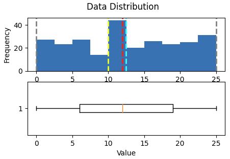
def show_distribution(var_data):
# Get statistics
min_val = var_data.min()
max_val = var_data.max()
mean_val = var_data.mean()
med_val = var_data.median()
mod_val = var_data.mode()[0]
print('Minimum:{:.2f} Mean:{:.2f} Median:{:.2f} Mode:{:.2f} Maximum:{:.2f} '.format(min_val,
mean_val,
med_val,
mod_val,
max_val))
fig, ax = plt.subplots(2, 1, figsize=(5,3))
# Plot hystogram
ax[0]. hist(var_data)
ax[0].set_ylabel('Frequency')
ax[0].axvline(x=min_val, color = 'gray', linestyle='dashed', linewidth = 2)
ax[0].axvline(x=mean_val, color = 'cyan', linestyle='dashed', linewidth = 2)
ax[0].axvline(x=med_val, color = 'red', linestyle='dashed', linewidth = 2)
ax[0].axvline(x=mod_val, color = 'yellow', linestyle='dashed', linewidth = 2)
ax[0].axvline(x=max_val, color = 'gray', linestyle='dashed', linewidth = 2)
# Plot boxplot
ax[1].boxplot(var_data, vert=False)
ax[1].set_xlabel('Value')
fig.suptitle('Data Distribution')
fig.show()
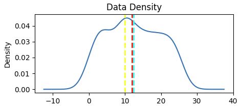
def show_density(var_data):
fig = plt.figure(figsize=(5,2))
var_data.plot.density()
plt.title('Data Density')
plt.axvline(x=var_data.mean(), color = 'cyan', linestyle='dashed', linewidth = 2)
plt.axvline(x=var_data.median(), color = 'red', linestyle='dashed', linewidth = 2)
plt.axvline(x=var_data.mode()[0], color = 'yellow', linestyle='dashed', linewidth = 2)
plt.show()
Add min clients columns if more than 7 clients were acquired.
Show distribution.
# Calculate what week got enough enoogh clients
min_clients = pd.Series(df_clients['Clients'] >= 7)
# Save who has enouugh clients
df_clients = pd.concat([df_clients, min_clients.rename("MinClients")], axis=1)
min_clients = pd.Series(df_clients['Clients'] >= 7)
# Save who has enouugh clients
df_clients = pd.concat([df_clients, min_clients.rename("MinClients")], axis=1)
var_data = df_clients['Clients']
show_distribution(var_data)
Result:
Minimum:0.00
Mean:12.43
Median:12.00
Mode:10.00
Maximum:25.00
Show density distribution
var_data = df_clients['Clients']
show_density(var_data)
Compute Variance & Standard variance
for col_name in ['Clients']:
col = df_clients[col_name]
rng = col.max() - col.min()
var = col.var()
std = col.std()
print(' {}: - Range: {:.2f} - Variance: {:.2f} - Std.Dev: {:.2f}'.format(col_name, rng, var, std))
col = df_clients[col_name]
rng = col.max() - col.min()
var = col.var()
std = col.std()
print(' {}: - Range: {:.2f} - Variance: {:.2f} - Std.Dev: {:.2f}'.format(col_name, rng, var, std))
Result:
Clients:
- Range: 25.00
- Variance: 54.24
- Std.Dev: 7.36
The standard deviation is generally the most useful.
It provides a measure of variance in the data on the same scale as the data itself .
The higher the standard deviation, the more variance there is when comparing values in the distribution to the distribution mean—in other words, the data is more spread out.
When working with a normal distribution, the standard deviation works with the particular characteristics of a normal distribution to provide even greater insight.
Finding the relationship between standard deviations and the data in the normal distribution.
import scipy.stats as stats
col = df_clients['Clients']
density = stats.gaussian_kde(col)
#Plot density
col.plot.density()
# Get mean and standrd deviation
s = col.std()
m = col.mean()
# Annotate 1 stdev
x1 = [m-s, m+s]
y1 = density(x1)
plt.plot(x1,y1, color='magenta')
plt.annotate('1 std (68.26%)', (x1[1],y1[1]))
# Annotate 2 stdevs
x2 = [m-(s*2), m+(s*2)]
y2 = density(x2)
plt.plot(x2,y2, color='green')
plt.annotate('2 std (95.45%)', (x2[1],y2[1]))
# Annotate 3 stdevs
x3 = [m-(s*3), m+(s*3)]
y3 = density(x3)
plt.plot(x3,y3, color='orange')
plt.annotate('3 std (99.73%)', (x3[1],y3[1]))
# Show the location of the mean
plt.axvline(col.mean(), color='cyan', linestyle='dashed', linewidth=1)
plt.axis('off')
plt.show()
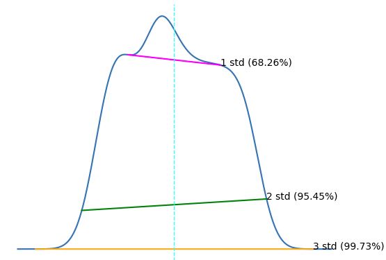
# Standard deviation means
# density(m) =0.042
# density (x1) = [0.037, 0,035].
# So +/-1mean: 0.042 = 100%, 0035 => 83.3%
# mean = 12.42, standard deviation = 7.26
# 68.26% are within range: 5.15 and 19.68 clients/week ( mean+/- 1 standard deviation: 12.42-7.26 = 5,15 and 12.42+7.26 = 19.68);
What we have above is the figure that describe Normal distribution, also known as Gaussian Distribution,
Gaussian distribution is ubiquitous in Data science.
It has a bell-shaped density curve described by meanand standard deviation
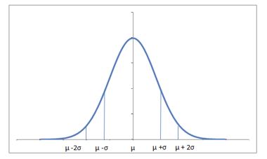
Almost 68% of the data falls within a distance of one standard deviation from the mean on either side and 95% within two standard deviations.
A Gaussian distribution withmean = 0 and standard deviation = 1 is called a standard normal distribution.
To generate a Gaussian distribution use:stats.gaussian_kde
References:
Statistical functions (scipy.stats) — SciPy v1.10.0 Manual
Probability Distribution | Formula, Types, & Examples (scribbr.com)
Probability Distributions in Python Tutorial | DataCamp