Study notes
Data exploration and analysis
It is an iterative process- analyse data and test hypotheses.
- Collect and clean data
- Apply statistical techniques to better understand data.
- Visualise data and determine relations.
- Check hypotheses and repeat the process.
Statistics
Science of collecting and analysing numerical data in large quantities, especially for the purpose of inferring proportions in a whole from those in a representative sample
It is is fundamentally about taking samples of data and using probability functions to extrapolateinformation about the full population of data.
Statistic samples
Data we have "in hand", avilable to be analysed.
Statistics population
All possible data we could collect (theoretical).
We can wish to have data from population but that's may not be possible in timeframe and amiable resources. However, we must estimate labels with the sample we have.
Havin enough samples we can calculate the Probability Density Function
Probability Density Function
Estimate distribution of labels for the full population
Ensemble Algorithm
Works by combining multiple base estimators to produce an optimal model,
Bagging(Essamble alghorytm)
Technique used in ML training models - Regression.
Combine multiple base estimators to produce an optimal model by applying an aggregate function to base collection.
Boosting (Essamble alghorytm)
Technique used in ML training models - Regression.
Create a sequence of models that build on one another to improve predictive performance.
Jupiter notebook
Popular way to tun basic script in web browser (no need python installed to run)
NumPy
Python library that gives functionality comparable with tools like MATLABS and R.
Simplify analyzing and manipulating data.
Matplotlib
Provides attractive data visualizations
Panda
Python library for data analysis and manipulation (excel for Python) - easy to use functionality for data tables.
Simplify analyzing and manipulating data.
Include basic functionality for visualization (graphs)
TensorFlow
Open-source platform for machine learning (end to end)
SciKit-learn
Offers simple and effective predictive data analysis
TensorFlow Software library for machine learning and artificial intelligence - focus on training and inference of deep neural networks.
Supply machine learning and deep learning capabilities
predict()
Predicts the actual class.
predict_proba()
Predicts the class probabilities.
DataFrame
Data structure that organizes data into a 2-dimensional table of rows and columns, much like a spreadsheet.
One of the most common data structures used in modern data analytics because they are a flexible and intuitive way of storing and working with data.
pandas.DataFrame.to_dict()
Convert the DataFrame to a dictionary.
The type of the key-value pairs can be customized with the parameters which determines the type of the values of the dictionary.
- ‘dict’ (default) :
dict like {column -> {index -> value}} - ‘list’ :
dict like {column -> [values]} - ‘series’ :
dict like {column -> Series(values)} - ‘split’ :
dict like {‘index’ -> [index], ‘columns’ -> [columns], ‘data’ -> [values]} - ‘tight’ :
dict like {‘index’ -> [index], ‘columns’ -> [columns], ‘data’ -> [values], ‘index_names’ -> [index.names], ‘column_names’ -> [column.names]} - ‘records’ :
list like [{column -> value}, … , {column -> value}] - ‘index’ :
dict like {index -> {column -> value}}
Pecentile
Give you a number that describes the value that a given percent of the values are lower than.
Quantile
A cut point, or line of division, that splits a probability distribution into continuous intervals with equal probabilities
Eliminate all values that fall below a specific percentile
Probability distribution
A function that accepts as input elements of some specific set x∈X, and produces as output, real-valued numbers between 0 and 1.
A probability distribution is a statistical function that describes all the possible values and probabilities for a random variable within a given range.
This range will be bound by the minimum and maximum possible values, but where the possible value would be plotted on the probability distribution will be determined by a number of factors. The mean (average), standard deviation, skewness, and kurtosis of the distribution are among these factors.
https://www.simplilearn.com/tutorials/statistics-tutorial/what-is-probability-distribution
Normalize data
Process data so values retain their proportional distribution, but are measured on the same scale
Proportional distribution
Distribute values across considering other factors
Example: Department intends to distribute funds for employment services across all areas of the state taking into consideration population distribution and client needs.
Correlation measurement
Quantify the relationship between these columns.
Outlier
A data point that is noticeably different from the rest
Regression
Where models predict a number, establishing a relationship between variables in the data that represent characteristics - known as the feature - of the thing being observed, and the variable we're trying to predict—known as the label
Supervised machine learning techniques involve training a model to operate on a set of features(x1,x2...xn) and predict a label (y) using a dataset that includes some already-known label values.
Mathematical approach to find the relationship between two or more variables
Regression works by establishing a relationship between variables in the data that represent characteristics—known as the features—of the thing being observed, and the variable we're trying to predict—known as the label
https://learn.microsoft.com/en-us/training/modules/train-evaluate-regression-models/2-what-is-regression
Linear regression
Simplest form of regression, with no limit to the number of features used.
Comes in many forms - often named by the number of features used and the shape of the curve that fits.
Decision trees
Take a step-by-step approach to predicting a variable.
If we think of our bicycle example, the decision tree may be first split examples between ones that are during Spring/Summer and Autumn/Winter, make a prediction based on the day of the week. Spring/Summer-Monday may have a bike rental rate of 100 per day, while Autumn/Winter-Monday may have a rental rate of 20 per day.
Ensemble algorithms
Construct a large number of trees - allowing better predictions on more complex data.
Ensemble algorithms, such as Random Forest, are widely used in machine learning and science due to their strong prediction abilities.
Hyperparameters
For real life scenarios with complex models and big datasets a model must befit repentantly (train, compare, adjust, train and so on...)
Values that change the way that the model is fit during loops.
Hyperparameter example Learning rate = sets how much a model is adjusted every cycle.
learning_rate - hyperparameter of GradientBoostingRegressorestimator.
n_estimators - Hyperparameter of GradientBoostingRegressorestimator.
Type:
- Discrete hyperparameter (select discrete values from continues distributions)
- qNormal distribution
- qUniformdistribution
- qLognormal distribution
- qLogUniform distribution
- Continuous hyperparameters
- Normal distribution
- Uniform distribution
- Lognormal distribution
- LogUniform distribution
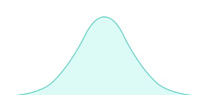
Normal distribution
Normal distribution or Gaussian distribution is a type of continuous probability distribution for a real-valued random variable
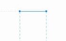
Uniform distribution
Continuous uniform distribution or rectangular distribution is a family of symmetric probability distributions. The distribution describes an experiment where there is an arbitrary outcome that lies between certain bounds.
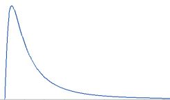
Lognormal distribution
Continuous probability distribution that models right-skewed data.
The lognormal distribution is related to logs and the normal distribution.
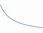
LogUniform distribution
Continuous probability distribution. It is characterised by its probability density function, within the support of the distribution, being proportional to the reciprocal of the variable.
Preprocess the Data
Perform some preprocessing of the data to make it easier for the algorithm to fit a model to it.
Scaling numeric features
Normalizing numeric features so they're on the same scale prevents features with large values from producing coefficients that disproportionately affect the predictions.
Bring all features values between 0 & 1, Ex 3 => 0.3, 480 => 0.48, 65=> 0.65
they're on the same scale. This prevents features with large values from producing coefficients that disproportionately affect the predictions
Encoding categorical variables
Convert categorical features into numeric representations
S,M,L => 0.1.2
by using a one hot encoding technique you can create individual binary (true/false) features for each possible category value.
Hot Encoding categorical variables
S M L
1 0 0
0 1 0
0 0 1
Classification
Form of machine learning in which you train a model to predict which category an item belongs to
Binary classification
is classification with two categories.
Regularization
technique that reduces error from a model by avoiding overfitting and training the model to function properly.
helps us control our model capacity, ensuring that our models are better at making (correct) classifications on data points that they were not trained on, which we call the ability to generalize.
threshold
A threshold value of 0.5 is used to decide whether the predicted label is a 1 (P(y) > 0.5) or a 0 (P(y) <= 0.5).
You can use the predict_proba method to see the probability pairs for each case
If we were to change the threshold, it would affect the predictions; and therefore change the metrics in the confusion matrix.
pipeline
Used extensively in machine learning, often to mean very different things.
1. Allow to define set of preprocessing steps that end with an algorithm.
Then fit entire pipeline to the data => model encapsulate all preprocessing steps and the (regression) algorithm.
Classification algorithms
logistic regression algorithm, (linear algorithm)
Support Vector Machine algorithms: Algorithms that define a hyperplane that separates classes.
Tree-based algorithms: Algorithms that build a decision tree to reach a prediction
Ensemble algorithms: Algorithms that combine the outputs of multiple base algorithms to improve generalizability (ex Random Forest)
Multiclass classification
Combination of multiple binary classifiers
One vs Rest (OVR)
Multiclass classification classifier.
A classifier is created for each possible class value, with a positive outcome for cases where the prediction is this class, and negative predictions for cases where the prediction is any other class
Ex:
square or not
circle or not
triangle or not
hexagon or not
One vs One (OVO)
Multiclass classification classifier
a classifier for each possible pair of classes is created. The classification problem with four shape classes would require the following binary classifiers:
square or circle
square or triangle
square or hexagon
circle or triangle
circle or hexagon
triangle or hexagon
predict_proba
Returns probabilities of a classification label.
Example:
Have a trained classification model
May run confusion_matrix(y_test, predictions) - check result
Run y_score =model.predict_proba(X_tests)
We get probability of 0 or 1 for every record in X_test
[[0.81651727 0.18348273]
[0.96298333 0.03701667]
[0.80862083 0.19137917]
...
[0.60688422 0.39311578]
[0.10672996 0.89327004]
[0.63865894 0.36134106]]
Stratification technique
Used (example in classification) when splitting the data to maintain the proportion of each label value in the training and validation datasets.
Clustering
Clustering is a form of unsupervised machine learning in which observations are grouped into clusters based on similarities in their data values, or features
process of grouping objects with similar objects
‘unsupervised’ method, where ‘training’ is done without labels
MinMaxScaler
Normalize the numeric features so they're on the same scale.
| # | area | perimeter | compactness | kernel_length | kernel_width | asymmetry_coefficient |
|---|---|---|---|---|---|---|
| 171 | 11.55 | 13.10 | 0.8455 | 5.167 | 2.845 | 6.715 |
| 58 | 15.38 | 14.77 | 0.8857 | 5.662 | 3.419 | 1.999 |
scaled_features = MinMaxScaler().fit_transform(features[data.columns[0:6]])
Result:array([[0.44098206, 0.50206612, 0.5707804 , 0.48648649, 0.48610121,
0.18930164],
[0.40509915, 0.44628099, 0.66243194, 0.36880631, 0.50106914,
0.03288302],
fit(data)
Method is used to compute the mean and std dev for a given feature to be used further for scaling.
transform(data)
Method is used toperform scaling using mean and std dev calculated using the .fit() method.
fit_transform()
Method does both fits and transform.
Principal Component Analysis (PCA)
Analyze the relationships between the features and summarize each observation as coordinates for two principal components
Translate the N-dimensional feature values into two-dimensional coordinates.
Within cluster sum of squares (WCSS) metric often used to measure this tightness
Lower values meaning that the data points are closer
k-means clustering algorithm
Iterative algorithm that tries to partition the dataset into Kpre-defined distinct non-overlapping subgroups (clusters) where each data point belongs to only one group.
The way kmeans algorithm works is as follows:
• The feature values are vectorized to define n-dimensional coordinates (where n is the number of features). In the flower example, we have two features (number of petals and number of leaves), so the feature vector has two coordinates that we can use to conceptually plot the data points in two-dimensional space.
• You decide how many clusters you want to use to group the flowers, and call this value k. For example, to create three clusters, you would use a k value of 3. Then k points are plotted at random coordinates. These points will ultimately be the center points for each cluster, so they're referred to as centroids.
• Each data point (in this case flower) is assigned to its nearest centroid.
• Each centroid is moved to the center of the data points assigned to it based on the mean distance between the points.
• After moving the centroid, the data points may now be closer to a different centroid, so the data points are reassigned to clusters based on the new closest centroid.
• The centroid movement and cluster reallocation steps are repeated until the clusters become stable or a pre-determined maximum number of iterations is reached.
KMeans.inertia_
Sum of Squared errors (SSE)
Calculates the sum of the distances of all points within a cluster from the centroid of the point. It is the difference between the observed value and the predicted value.
The K-means algorithm aims to choose centroids that minimize the inertia, or within-cluster sum-of-squares criterion. Inertia can be recognized as a measure of how internally coherent clusters are.
PyTorch
PyTorch
Machine learning framework based on the Torch library, used for applications such as computer vision and natural language processing (NLP)
Supply machine learning and deep learning capabilities
An open source machine learning framework that accelerates the path from research prototyping to production deployment
PyTorch datasets - the data is stored in PyTorch *tensor* objects.
manual_seed(torch.manual_seed())
Sets the seed for generating random numbers.
Returns a torch.Generator object.
optimizer.zero_grad()
In PyTorch, for every mini-batch during the training phase, we typically want to explicitly set the gradients to zero before starting to do backpropragation (i.e., updating the Weights and biases) because PyTorch accumulates the gradients on subsequent backward passes.
Because of this, when you start your training loop, ideally you should zero out the gradients so that you do the parameter update correctly
Hierarchical Clustering
clustering algorithm in which clusters themselves belong to a larger group, which belong to even larger groups, and so on. The result is that data points can be clusters in differing degrees of precision: with a large number of very small and precise groups, or a small number of larger groups.
Useful for not only breaking data into groups, but understanding the relationships between these groups.
A major advantage of hierarchical clustering is that it does not require the number of clusters to be defined in advance, and can sometimes provide more interpretable results than non-hierarchical approaches.
The major drawback is that these approaches can take much longer to compute than simpler approaches and sometimes are not suitable for large datasets.
divisive method
Hierarchical Clustering
"top down" approach starting with the entire dataset and then finding partitions in a stepwise manner
agglomerative method
Hierarchical Clustering
"bottom up** approach. In this lab you will work with agglomerative clustering which roughly works as follows:
1. The linkage distances between each of the data points is computed.
2. Points are clustered pairwise with their nearest neighbor.
3. Linkage distances between the clusters are computed.
4. Clusters are combined pairwise into larger clusters.
5. Steps 3 and 4 are repeated until all data points are in a single cluster.
linkage function
Hierarchical Clustering - agglomerative method
can be computed in a number of ways:
• Ward linkage measures the increase in variance for the clusters being linked,
• Average linkage uses the mean pairwise distance between the members of the two clusters,
• Complete or Maximal linkage uses the maximum distance between the members of the two clusters.
Several different distance metrics are used to compute linkage functions:
• Euclidian or l2 distance is the most widely used. This metric is only choice for the Ward linkage method - measures of difference
• Manhattan or l1 distance is robust to outliers and has other interesting properties - measures of difference
• Cosine similarity, is the dot product between the location vectors divided by the magnitudes of the vectors. - measure of similarity
Similarity can be quite useful when working with data such as images or text documents.
Deep learning
Advanced form of machine learning that tries to emulate the way the human brain learns.
1. When the first neuron in the network is stimulated, the input signal is processed
2. If it exceeds a particular threshold, the neuron is activated and passes the signal on to the neurons to which it is connected.
3. These neurons in turn may be activated and pass the signal on through the rest of the network.
4. Over time, the connections between the neurons are strengthened by frequent use as you learn how to respond effectively.
Deep learning emulates this biological process using artificial neural networks that process numeric inputs rather than electrochemical stimuli.
The incoming nerve connections are replaced by numeric inputs that are typically identified as x (x1,x2…)
Associated with each x value is a weight (w)
Additionally, a bias (b) input is added to enable fine-grained control over the network
The neuron itself encapsulates a function that calculates a weighted sum of x, w, and b. This function is in turn enclosed in an activation function that constrains the result (often to a value between 0 and 1) to determine whether or not the neuron passes an output onto the next layer of neurons in the network.
Deep neural network
DNN model
The deep neural network model for the classifier consists of multiple layers of artificial neurons. In this case, there are four layers:
• An input layer with a neuron for each expected input (x) value.
• Two so-called hidden layers, each containing five neurons.
• An output layer containing three neurons - one for each class probability (y) value to be predicted by the model.
Particularly useful for dealing with data that consists of large arrays of numeric values - such as images.
Are the foundation for an area artificial intelligence called computer vision,
epochs
Training DNN model
The training process for a deep neural network consists of multiple iterations
backpropagation
Training DNN model
the loss from the model is calculated and used to adjust the weight and bias values
Calculating loss
Training DNN model
The loss is calculated using a function, which operates on the results from the final layer of the network, which is also a function
multiple observations, we typically aggregate the variance
Loss function
Training DNN model
the entire model from the input layer right through to the loss calculation is just one big nested function
Functions have a few really useful characteristics, including:
• You can conceptualize a function as a plotted line comparing its output with each of its variables.
• You can use differential calculus to calculate the derivative of the function at any point with respect to its variables.
The derivative of a function for a given point indicates whether the slope (or gradient) of the function output (in this case, loss) is increasing or decreasing with respect to a function variable (in this case, the weight value).
A positive derivative indicates that the function is increasing, and a negative derivative indicates that it is decreasing.
optimizer
apply this same trick for all of the weight and bias variables in the model and determine in which direction we need to adjust them (up or down) to reduce the overall amount of loss in the model.
There are multiple commonly used optimization algorithms:
- stochastic gradient descent (SGD),
- Adaptive Learning Rate (ADADELTA),
- Adaptive Momentum Estimation (Adam), and others;
All of which are designed to figure out how to adjust the weights and biases to minimize loss.
Learning rate
how much should the optimizer adjust the weights and bias values
A low learning rate results in small adjustments (so it can take more epochs to minimize the loss), while a high learning rate results in large adjustments (so you might miss the minimum altogether).
Convolutional neural networks (CNN)
A CNN typically works by extracting features from images, and then feeding those features into a fully connected neural network to generate a prediction.
CNNs consist of multiple layers, each performing a specific task in extracting features or predicting labels.
The feature extraction layers in the network have the effect of reducing the number of features from the potentially huge array of individual pixel values to a smaller feature set that supports label prediction.
1. An image is passed to the convolutional layer. In this case, the image is a simple geometric shape.
2. The image is composed of an array of pixels with values between 0 and 255 (for color images, this is usually a 3-dimensional array with values for red, green, and blue channels).
3. A filter kernel is generally initialized with random weights (in this example, we've chosen values to highlight the effect that a filter might have on pixel values; but in a real CNN, the initial weights would typically be generated from a random Gaussian distribution). This filter will be used to extract a feature map from the image data.
4. The filter is convolved across the image, calculating feature values by applying a sum of the weights multiplied by their corresponding pixel values in each position. A Rectified Linear Unit (ReLU) activation function is applied to ensure negative values are set to 0.
5. After convolution, the feature map contains the extracted feature values, which often emphasize key visual attributes of the image. In this case, the feature map highlights the edges and corners of the triangle in the image.
overlay
An image is also just a matrix of pixel values. To apply the filter, you "overlay" it on an image and calculate a weighted sum of the corresponding image pixel values under the filter kernel. The result is then assigned to the center cell of an equivalent 3x3 patch in a new matrix of values that is the same size as the image
Pooling layers
After extracting feature values from images, pooling (or downsampling) layers are used to reduce the number of feature values while retaining the key differentiating features that have been extracted.
One of the most common kinds of pooling is max pooling in which a filter is applied to the image, and only the maximum pixel value within the filter area is retained. So for example, applying a 2x2 pooling kernel to the following patch of an image would produce the result 155.
1. The feature map extracted by a filter in a convolutional layer contains an array of feature values.
2. A pooling kernel is used to reduce the number of feature values. In this case, the kernel size is 2x2, so it will produce an array with quarter the number of feature values.
3. The pooling kernel is convolved across the feature map, retaining only the highest pixel value in each position.
overfitting
the resulting model performs well with the training data but doesn't generalize well to new data on which it wasn't trained.
One technique you can use to mitigate overfitting is to include layers in which the training process randomly eliminates (or "drops") feature maps
Other techniques you can use to mitigate overfitting include randomly flipping, mirroring, or skewing the training images to generate data that varies between training epochs.
- For this reason, it’s common to use some kind of regularisation method to prevent the model from fitting too closely to the training data
Flattening layers
resulting feature maps are multidimensional arrays of pixel values. A flattening layer is used to flatten the feature maps into a vector of values that can be used as input to a fully connected layer.
CNN architecture 1. Images are fed into a convolutional layer. In this case, there are two filters, so each image produces two feature maps.
2. The feature maps are passed to a pooling layer, where a 2x2 pooling kernel reduces the size of the feature maps.
3. A dropping layer randomly drops some of the feature maps to help prevent overfitting.
4. A flattening layer takes the remaining feature map arrays and flattens them into a vector.
5. The vector elements are fed into a fully connected network, which generates the predictions. In this case, the network is a classification model that predicts probabilities for three possible image classes (triangle, square, and circle).
Transfer learning
Conceptually, this neural network consists of two distinct sets of layers:
1. A set of layers from the base model that perform feature extraction.
extraction layers apply convolutional filters and pooling to emphasize edges, corners, and other patterns in the images that can be used to differentiate them, and in theory should work for any set of images with the same dimensions as the input layer of the network
2. A fully connected layer that takes the extracted features and uses them for class prediction.
extraction layers apply convolutional filters and pooling to emphasize edges, corners, and other patterns in the images that can be used to differentiate them, and in theory should work for any set of images with the same dimensions as the input layer of the network
This approach enables you to keep the pre-trained weights for the feature extraction layers, which means you only need to train the prediction layers you have added.
Azure Machine Learning studio
Cloud-based service that helps simplify some of the tasks it takes to prepare data, train a model, and deploy a predictive service.
Azure Machine Learning workspace
Resource in your Azure subscription you use to manage data, compute resources, code, models, and other artifacts related to your machine learning workloads.
Azure Machine Learning compute
Cloud-based resources on which you can run model training and data exploration processes.
1. Compute Instances: Development workstations that data scientists can use to work with data and models.
2. Compute Clusters: Scalable clusters of virtual machines for on-demand processing of experiment code.
3. Inference Clusters: Deployment targets for predictive services that use your trained models.
4. Attached Compute: Links to existing Azure compute resources, such as Virtual Machines or Azure Databricks clusters.
Azure Machine Learning
Service for training and managing machine learning models, for which you need compute on which to run the training process.
Azure Automated Machine Learning
Automatically tries multiple pre-processing techniques and model-training algorithms in parallel.
These automated capabilities use the power of cloud compute to find the best performing supervised machine learning model for your data.
It provides a way to save time and resources by automating algorithm selection and hyperparameter tuning.
AutoML process
1. Prepare data: Identify the features and label in a dataset. Pre-process, or clean and transform, the data as needed.
2. Train model: Split the data into two groups, a training and a validation set. Train a machine learning model using the training data set. Test the machine learning model for performance using the validation data set.
3. Evaluate performance: Compare how close the model's predictions are to the known labels.
4. Deploy a predictive service: After you train a machine learning model, you can deploy the model as an application on a server or device so that others can use it.
Train model
You can use automated machine learning to train models for:
• Classification (predicting categories or classes)
• Regression (predicting numeric values)
• Time series forecasting (predicting numeric values at a future point in time)
In Automated Machine Learning, you can select configurations for the primary metric, type of model used for training, exit criteria, and concurrency limits.
Evaluate performance
After the job has finished you can review the best performing model.
Inference Clusters
Deployment targets for predictive services that use your trained models
Pipelines
Let you organize, manage, and reuse complex machine learning workflows across projects and users. A pipeline starts with the dataset from which you want to train the model
Components
Encapsulates one step in a machine learning pipeline
Azure Machine Learning Jobs
executes a task against a specified compute target
Stratified sampeling
technique used in Machine Learning to generate a test set
Random sampling is generally fine if the original dataset is large enough; if not, a bias is introduced due to the sampling error. Stratified Sampling is a sampling method that reduces the sampling error in cases where the population can be partitioned into subgroups.
We perform Stratified Sampling by dividing the population into homogeneous subgroups, called strata, and then applying Simple Random Sampling within each subgroup.
As a result, the test set is representative of the population, since the percentage of each stratum is preserved. The strata should be disjointed; therefore, every element within the population must belong to one and only one stratum.
ML experiment
• a named process, usually the running of a script or a pipeline, that can generate metrics and outputs and be tracked in the Azure Machine Learning workspace
• it can be run multiple times, with different data, code, or settings; and Azure Machine Learning tracks each run, enabling you to view run history and compare results for each run.
• When you submit an experiment, you use its run context to initialize and end the experiment run that is tracked in Azure Machine Learning
1. Every experiment generates log files (keep data between runs)
2. You can view the metrics logged by an experiment run in Azure Machine Learning studio or by using the RunDetails widget in a notebook
3. In addition to logging metrics, an experiment can generate output files. The output files of an experiment are saved in its outputs folder.
experiment script
• a Python code file that contains the code you want to run in the experiment
1. To access the experiment run context (which is needed to log metrics) the script must import the azureml.core.Run class and call its get_context method.
2. To run a script as an experiment, you must define
a. a script configuration that defines the script to be run and
b. the Python environment in which to run it.
This is implemented by using a ScriptRunConfig object.
Log experiment metrics
Run object
Every experiment generates log files that include the messages that would be written to the terminal during interactive execution.
If you want to record named metrics for comparison across runs, you can do so by using the Run object; which provides a range of logging functions specifically for this purpose. These include:
• log: Record a single named value.
• log_list: Record a named list of values.
• log_row: Record a row with multiple columns.
• log_table: Record a dictionary as a table.
• log_image: Record an image file or a plot.
Environment
Defines Python packages, environment variables, and Docker settings that are used in machine learning experiments, including in data preparation, training, and deployment to a web service.
An Environment is managed and versioned in an Azure Machine Learning Workspace.
You can update an existing environment and retrieve a version to reuse.
Environments are exclusive to the workspace they are created in and can't be used across different workspaces.
Azure Machine Learning provides curated environments, which are predefined environments that offer good starting points for building your own environments. Curated environments are backed by cached Docker images, providing a reduced run preparation cost.
Environment are created in by:
- Initialize a new Environment object.
- Use one of the Environment class methods: from_conda_specification, from_pip_requirements, or from_existing_conda_environment.
- Use the submit method of the Experiment class to submit an experiment run without specifying an environment, including with an Estimator object.
To use parameters in a script, you must use a library such as argparse to read the arguments passed to the script and assign them to variables.
train_test_split sklearn
split model
LogisticRegression
Supervised classification algorithm.
The model builds a regression model to predict the probability that a given data entry belongs to the category numbered as “1” or "0"
Linear regression assumes that the data follows a linear function, Logistic regression models the data using the sigmoid function.
Hyperparameter
- configure how the model is trained
- top-level parameters that control the learning process and the model parameters that result from it. As a machine learning engineer designing a model, you choose and set hyperparameter values that your learning algorithm will use before the training of the model even begins
Regularization rate
(regression algorithm)
The Logistic regression function, which originally takes training data X, and label yas input, now needs to add one more input: the strength of regularization λ.
used to train models that generalize better on unseen data,by preventing the algorithm from overfitting the training dataset.
Hyperparameter
search space
Search space for hyperparameters values
To define a search space for hyperparameter tuning, create a dictionary with the appropriate parameter expression for each named hyperparameter
The specific values used in a hyperparameter tuning run depend on the type of sampling used.
Discrete hyperparameters
distributions
• qnormal
• quniform
• qlognormal
• qloguniform
Continuous hyperparameters
Distributions
• normal
• uniform
• lognormal
• loguniform
Hyperparameters search space
values sampling
Grid sampling - can only be employed when all hyperparameters are discrete, and is used to try every possible combination of parameters in the search space.
Random sampling is used to randomly select a value for each hyperparameter, which can be a mix of discrete and continuous values
Bayesian sampling chooses hyperparameter values based on the Bayesian optimization algorithm, which tries to select parameter combinations that will result in improved performance from the previous selection.
Training early termination
set an early termination policy that abandons runs that are unlikely to produce a better result than previously completed runs.
The policy is evaluated at an evaluation_interval you specify, based on each time the target performance metric is logged.
You can also set a delay_evaluation parameter to avoid evaluating the policy until a minimum number of iterations have been completed.
Data privacy parameters
The amount of variation caused by adding noise is configurable
epsilon This value governs the amount of additional risk that your personal data can be identified through rejecting the opt-out option and participating in a study
- A low epsilon value provides the most privacy, at the expense of less accuracy when aggregating the data
- A higher epsilon value results in aggregations that are more true to the actual data distribution, but in which the individual contribution of a single individual to the aggregated value is less obscured by noise - less privacy
Differential privacy
Technique that is designed to preserve the privacy of individual data points by adding "noise" to the data. The goal is to ensure that enough noise is added to provide privacy for individual values while ensuring that the overall statistical makeup of the data remains consistent, and aggregations produce statistically similar results as when used with the original raw data.
The noise is different for each analysis, so the results are non-deterministic – in other words, two analyses that perform the same aggregation may produce slightly different results.
The amount of variation caused by adding noise is configurable through a parameter called epsilon
- A low epsilon value provides the most privacy, at the expense of less accuracy when aggregating the data.
- A higher epsilon value results in aggregations that are more true to the actual data distribution, but in which the individual contribution of a single individual to the aggregated value is less obscured by noise.
Create an analysis in which noise is added to the source data.
The underlying mathematics of how the noise is added can be quite complex, but SmartNoise takes care of most of the details for you.
- Upper and lower bounds
Clampingis used to set upper and lower bounds on values for a variable. This is required to ensure that the noise generated by SmartNoise is consistent with the expected distribution of the original data. - Sample size
To generate consistent differentially private data for some aggregations, SmartNoise needs to know the size of the data sample to be generated. - Epsilon
Put simplistically, epsilon is a non-negative value that provides an inverse measure of the amount of noise added to the data. A low epsilon results in a dataset with a greater level of privacy, while a high epsilon results in a dataset that is closer to the original data. Generally, you should use epsilon values between 0 and 1. Epsilon is correlated with another value named delta, that indicates the probability that a report generated by an analysis is not fully private.
Covariance
Establish relationships between variables.
Positive values - one feature increases, the second increases the same; direct relation.
Model explainers
Use statistical techniques to calculate feature importance.
Allow to quantify the relative influence each feature in the training dataset has on label prediction.
Explainers work by evaluating a test data set of feature cases and the labels the model predicts for them.
Global feature importance
quantifies the relative importance of each feature in the test dataset as a whole
It provides a general comparison of the extent to which each feature in the dataset influences prediction.
model-agnostic
Use ML models to study the the underlying structure without assuming that it can be accurately described by the model because of its nature.
Local feature importance
measures the influence of each feature value for a specific individual prediction.
For a regression model, there are no classes so the local importance values simply indicate the level of influence each feature has on the predicted scalar label.
MimicExplainer
Model explainers
An explainer that creates a global surrogate model that approximates your trained model and can be used to generate explanations.
This explainable model must have the same kind of architecture as your trained model (for example, linear or tree-based).
TabularExplainer
Model explainers
An explainer that acts as a wrapper around various SHAP explainer algorithms, automatically choosing the one that is most appropriate for your model architecture.
Model explainers
a Permutation Feature Importance explainer that analyzes feature importance by shuffling feature values and measuring the impact on prediction performance.
SHAP
SHapley Additive exPlanations — is probably the state of the art in Machine Learning explain ability.
In a nutshell, SHAP values are used whenever you have a complex model (could be a gradient boosting, a neural network, or anything that takes some features as input and produces some predictions as output) and you want to understand what decisions the model is making.
Disparity
a difference in level or treatment, especially one that is seen as unfair.
In prediction it is about fairness of the model
Measuring disparity in predictions
One way to start evaluating the fairness of a model is to compare predictions for each group within a sensitive feature.
To evaluate the fairness of a model, you can apply the same predictive performance metric to subsets of the data, based on the sensitive features on which your population is grouped, and measure the disparity in those metrics across the subgroups.
Potential causes of disparity • Data imbalance.
• Indirect correlation
• Societal biases.
Data imbalance
Some groups may be overrepresented in the training data, or the data may be skewed so that cases within a specific group aren't representative of the overall population.
Indirect correlation
The sensitive feature itself may not be predictive of the label, but there may be a hidden correlation between the sensitive feature and some other feature that influences the prediction. For example, there's likely a correlation between age and credit history, and there's likely a correlation between credit history and loan defaults. If the credit history feature is not included in the training data, the training algorithm may assign a predictive weight to age without accounting for credit history, which might make a difference to loan repayment probability.
Societal biases
Subconscious biases in the data collection, preparation, or modeling process may have influenced feature selection or other aspects of model design.
Fairlearn
Python package that you can use to analyze models and evaluate disparity between predictions and prediction performance for one or more sensitive features.
The mitigation support in Fairlearn is based on the use of algorithms to create alternative models that apply parity constraints to produce comparable metrics across sensitive feature groups. Fairlearn supports the following mitigation techniques.
Exponentiated Gradient
Fairlearn techniques
A reduction technique that applies a cost-minimization approach to learning the optimal trade-off of overall predictive performance and fairness disparity
- Binary classification
- Regression
Grid Search
Fairlearn techniques
A simplified version of the Exponentiated Gradient algorithm that works efficiently with small numbers of constraints
- Binary classification
- Regression
Threshold Optimizer
Fairlearn techniques
A post-processing technique that applies a constraint to an existing classifier, transforming the prediction as appropriate
- Binary classification
Fairlearn constraints
• Demographic parity
Use this constraint with any of the mitigation algorithms to minimize disparity in the selection rate across sensitive feature groups. For example, in a binary classification scenario, this constraint tries to ensure that an equal number of positive predictions are made in each group.
• True positive rate parity:
Use this constraint with any of the mitigation algorithms to minimize disparity in true positive rate across sensitive feature groups. For example, in a binary classification scenario, this constraint tries to ensure that each group contains a comparable ratio of true positive predictions.
• False-positive rate parity:
Use this constraint with any of the mitigation algorithms to minimize disparity in false_positive_rate across sensitive feature groups. For example, in a binary classification scenario, this constraint tries to ensure that each group contains a comparable ratio of false-positive predictions.
• Equalized odds:
Use this constraint with any of the mitigation algorithms to minimize disparity in combined true positive rate and false_positive_rate across sensitive feature groups. For example, in a binary classification scenario, this constraint tries to ensure that each group contains a comparable ratio of true positive and false-positive predictions.
• Error rate parity:
Use this constraint with any of the reduction-based mitigation algorithms (Exponentiated Gradient and Grid Search) to ensure that the error for each sensitive feature group does not deviate from the overall error rate by more than a specified amount.
• Bounded group loss:
Use this constraint with any of the reduction-based mitigation algorithms to restrict the loss for each sensitive feature group in a regression model.
data drift
change in data profiles between training and inferencing and over the time.
To monitor data drift using registered datasets, you need to register two datasets:
- A baseline dataset - usually the original training data.
- A target dataset that will be compared to the baseline based on time intervals. This dataset requires a column for each feature you want to compare, and a timestamp column so the rate of data drift can be measured.
Service tags
a group of IP address prefixes from a given Azure service
Microsoft manages the address prefixes encompassed by the service tag and automatically updates the service tag as addresses change, minimizing the complexity of frequent updates to network security rules.
You can use service tags in place of specific IP addresses when you create security rules to define network access controls on network security groups or Azure Firewall.
Azure VNet
the fundamental building block for your private network in Azure. VNet enables Azure resources, such as Azure Blob Storage and Azure Container Registry, to securely communicate with each other, the internet, and on-premises networks.
With a VNet, you can enhance security between Azure resources and filter network traffic to ensure only trusted users have access to the network.
IP address space:
When creating a VNet, you must specify a custom private IP address space using public and private (RFC 1918) addresses.
Subnets
enable you to segment the virtual network into one or more sub-networks and allocate a portion of the virtual network's address space to each subnet, enhancing security and performance.
Network interfaces (NIC)
the interconnection between a VM and a virtual network (VNet). When you create a VM in the Azure portal, a network interface is automatically created for you.
Network security groups (NSG)
can contain multiple inbound and outbound security rules that enable you to filter traffic to and from resources by source and destination IP address, port, and protocol.
Load balancers
can be configured to efficiently handle inbound and outbound traffic to VMs and VNets, while also offering metrics to monitor the health of VMs.
Service endpoints
provide the identity of your virtual network to the Azure service.
Service endpoints use public IP addresses
Once you enable service endpoints in your virtual network, you can add a virtual network rule to secure the Azure service resources to your virtual network.
Private endpoints
effectively bringing the Azure services into your VNet
Private endpoint uses a private IP address from your VNet
network interfaces that securely connect you to a service powered by Azure Private Link
Private Link Service
your own service, powered by Azure Private Link that runs behind an Azure Standard Load Balancer, enabled for Private Link access. This service can be privately connected with and consumed using Private Endpoints deployed in the user's virtual network
Azure VPN gateway
Connects on-premises networks to the VNet over a private connection. Connection is made over the public internet. There are two types of VPN gateways that you might use:
• Point-to-site: Each client computer uses a VPN client to connect to the VNet.
• Site-to-site: A VPN device connects the VNet to your on-premises network.
ExpressRoute
Connects on-premises networks into the cloud over a private connection. Connection is made using a connectivity provider.
Azure Bastion
In this scenario, you create an Azure Virtual Machine (sometimes called a jump box) inside the VNet. You then connect to the VM using Azure Bastion. Bastion allows you to connect to the VM using either an RDP or SSH session from your local web browser. You then use the jump box as your development environment. Since it is inside the VNet, it can directly access the workspace.
Azure Databricks
Microsoft analytics service, part of the Microsoft Azure cloud platform. It offers an integration between Microsoft Azure and the Apache Spark's Databricks implementation
notebook
a document that contains runnable code, descriptive text, and visualizations.
We can override the default language by specifying the language magic command %<language> at the beginning of a cell.
The supported magic commands are:
• %python
• %r
• %scala
• %sql
Notebooks also support a few auxiliary magic commands:
• %sh: Allows you to run shell code in your notebook
• %fs: Allows you to use dbutils filesystem commands
• %md: Allows you to include various types of documentation, including text, images, and mathematical formulas and equations.
workspace
It groups objects (like notebooks, libraries, experiments) into folders,
Provides access to your data,
Provides access to the computations resources used (clusters, jobs).
cluster
set of computational resources on which you run your code (as notebooks or jobs). We can run ETL pipelines, or machine learning, data science, analytics workloads on the cluster.
• An all-purpose cluster. Multiple users can share such clusters to do collaborative interactive analysis.
• A jbto run a specific job. The cluster will be terminated when the job completes (A job is a way of running a notebook or JAR either immediately or on a scheduled basis).
job
a way of running a notebook or JAR either immediately or on a scheduled basis
Databricks runtimes
the set of core components that run on Azure Databricks clusters.
Azure Databricks offers several types of runtimes:
Databricks Runtime: includes Apache Spark, components and updates that optimize the usability, performance, and security for big data analytics.
Databricks Runtime for Machine Learning: a variant that adds multiple machine learning libraries such as TensorFlow, Keras, and PyTorch.
Databricks Light: for jobs that don’t need the advanced performance, reliability, or autoscaling of the Databricks Runtime.
Azure Databricks database
a collection of tables. An Azure Databricks table is a collection of structured data.
We can cache, filter, and perform any operations supported by Apache Spark DataFrames on Azure Databricks tables. We can query tables with Spark APIs and Spark SQL.
Databricks File System (DBFS)
distributed file system mounted into a Databricks workspace and available on Databricks clusters. DBFS is an abstraction on top of scalable object storage and offers the following benefits:
• Allows you to mount storage objects so that you can seamlessly access data without requiring credentials.
• Allows you to interact with object storage using directory and file semantics instead of storage URLs.
• Persists files to object storage, so you won’t lose data after you terminate a cluster.
Resilient Distributed Dataset (RDD)
The fundamental data structure of Apache Spark which are an immutable collection of objects which computes on the different node of the cluster.
Each and every dataset in Spark RDD is logically partitioned across many servers so that they can be computed on different nodes of the cluster.
MLLib
SAME LIBRARY as Spark ML
legacy approach for machine learning on Apache Spark. It builds off of Spark's Resilient Distributed Dataset (RDD) data structure.
additional data structures on top of the RDD, such as DataFrames, have reduced the need to work directly with RDDs.
classic" MLLib namespace is org.apache.spark.mllib
Spark ML
SAME LIBRARY as MLLib
Primary library for machine learning development in Apache Spark.
It supports DataFrames in its API (versus the classic RDD approach).
USE this as much as you can This makes Spark ML an easier library to work with for data scientists .
As Spark DataFrames share many common ideas with the DataFrames used in Pandas and R.
Spark ML workspace is org.apache.spark.ml.
Train and validate a model
The process of training and validating a machine learning model using Spark ML is fairly straightforward. The steps are as follows:
• Splitting data.
• Training a model.
• Validating a model.
Splitting data
splitting data between training and validation datasets
This hold-out dataset can be useful for determining whether the training model is overfitting
DataFrames support a randomSplit() method, which makes this process of splitting data simple
Training a model
Training a model relies on three key abstractions:
• a transformer - performing feature engineering and feature selection, as the result of a transformer is another DataFrame - support a randomSplit()
• an estimator - takes a DataFrame as an input and returns a model. It takes a DataFrame as an input and returns a model, which is itself a transformer.
ex: LinearRegression
It accepts a DataFrame and produces a Model. Estimators implement a .fit() method.
• a pipeline - combine together estimators and transformers and implement a .fit()
Validating a model
process based on built-in summary statistics
the model contains a summary object, which includes scores such as Root Mean Square Error (RMSE), Mean Absolute Error (MAE), and coefficient of determination (R2, pronounced R-squared)
with a validation dataset, it is possible to calculate summary statistics on a never-before-seen set of data, running the model's transform() function against the validation dataset.
other machine learning frameworks
Azure Databricks supports machine learning frameworks other than Spark ML and MLLib.
For libraries, which do not support distributed training, it is also possible to use a single node cluster. For example, PyTorch and TensorFlow both support single node use.
DataFrames
the distributed collections of data, organized into rows and columns. Each column in a DataFrame has a name and an associated type.
Spark DataFrames can be created from various sources, such as CSV files, JSON, Parquet files, Hive tables, log tables, and external databases.
Query dataframes
Spark SQL is a component that introduced the DataFrames, which provides support for structured and semi-structured data.
Spark has multiple interfaces (APIs) for dealing with DataFrames:
• the .sql() method, which allows to run arbitrary SQL queries on table data.
• use the Spark domain-specific language for structured data manipulation, available in Scala, Java, Python, and R.
DataFrame API
The Apache Spark DataFrame API provides a rich set of functions (select columns, filter, join, aggregate, and so on) that allow you to solve common data analysis problems efficiently. A complex operation where tables are joined, filtered, and restructured is easy to write, easy to understand, type safe, feels natural for people with prior sql experience
statistics about the DataFrame • Available statistics are:
• Count
• Mean
• Stddev
• Min
• Max
• Arbitrary approximate percentiles specified as a percentage (for example, 75%).
Plot options
• The following display options are available:
• We can choose the DataFrame columns to be used as axes (keys, values).
• We can choose to group our series of data.
• We can choose the aggregations to be used with our grouped data (avg, sum, count, min, max).
Machine learning
Data science technique used to extract patterns from data allowing computers to identify related data, forecast future outcomes, behaviors, and trends.
In machine learning, you train the algorithm with data and answers, also known as labels, and the algorithm learns the rules to map the data to their respective labels.
Synthetic Minority Over-sampling Technique (SMOTE)
Oversampling technique that allows us to generate synthetic samples for our minority categories
the idea is based on the K-Nearest Neighbors algorithm
We get a difference between a sample and one of its k nearest neighbours and multiply by some random value in the range of (0, 1). Finally, we generate a new synthetic sample by adding the value we get from the previous operation
Imputation of null values
Null values refer to unknown or missing data. Strategies for dealing with this scenario include:
• Dropping these records: Works when you do not need to use the information for downstream workloads.
• Adding a placeholder (for example, -1): Allows you to see missing data later on without violating a schema.
• Basic imputing: Allows you to have a "best guess" of what the data could have been, often by using the mean or median of non-missing data for numerical data type, or most_frequent value of non-missing data for categorical data type.
• Advanced imputing: Determines the "best guess" of what data should be using more advanced strategies such as clustering machine learning algorithms or oversampling techniques such as SMOTE (Synthetic Minority Over-sampling Technique).
ScriptRunConfig
To submit a run, create a configuration object that describes how the experiment is run. ScriptRunConfig is an examples of configuration objects used.
Identifies the Python script file to be run in the experiment. An experiment can be run based on it.
The ScriptRunConfig also determines the compute target and Python environment.
data cleaning
Imputation of null values, Imputation of null values, Duplicate records, Outliers
feature engineering
process of generating new predictive features from existing raw data
it is important to derive features from existing raw data that better represent the nature of the data and thus help improve the predictive power of the machine learning algorithms
• Aggregation (count, sum, average, mean, median, and the like)
• Part-of (year of date, month of date, week of date, and the like)
• Binning (grouping entities into bins and then applying aggregations)
• Flagging (boolean conditions resulting in True of False)
• Frequency-based (calculating the frequencies of the levels of one or more categorical variables)
• Embedding (transforming one or more categorical or text features into a new set of features, possibly with a different cardinality)
• Deriving by example
data scaling
Bring features to similar scales
There are two common approaches to scaling numerical features:
• Normalization - mathematically rescales the data into the range [0, 1].
• Standardization - rescales the data to have mean = 0 and standard deviation = 1
For the numeric input
- compute the mean and standard deviation using all the data available in the training dataset.
- then for each individual input value, you scale that value by subtracting the mean and then dividing by the standard deviation.
data encoding
converting data into a format required for a number of information processing needs
We will look at two common approaches for encoding categorical data:
• Ordinal encoding - converts categorical data into integer codes ranging from 0 to (number of categories – 1).
• One-hot encoding - transforming each categorical value into n (= number of categories) binary values, with one of them 1, and all others 0 (recommended)
MLflow
Open-source product designed to manage the Machine Learning development lifecycle.
Allows data scientists to train models, register those models, deploy the models to a web server, and manage model updates.
Important part of machine learning with Azure Databricks, as it integrates key operational processes with the Azure Databricks interface (also operate on workloads outside of Azure Databricks)
Offers a standardized format for packaging models for distribution.
Components:
• MLflow Tracking - provides the ability to audit the results of prior model training executions. It is built around runs
• MLflow Projects - a way of packaging up code in a manner, which allows for consistent deployment and the ability to reproduce results
• MLflow Models - standardized model format allows MLflow to work with models generated from several popular libraries, including scikit-learn, Keras, MLlib, ONNX, and more
• MLflow Model Registry - llows data scientists to register models in a registry
Key steps:
• Mode registration - stores the details of a model in the MLflow Model Registry, along with a name for ease of access
• Model Versioning - makes model management easy by labeling new versions of models and retaining information on prior model versions automatically
MLflow Tracking
To use MLflow to track metrics for an inline experiment, you must set the MLflow tracking URI to the workspace where the experiment is being run. This enables you to use mlflow tracking methods to log data to the experiment run.
When you use MLflow tracking in an Azure ML experiment script, the MLflow tracking URI is set automatically when you start the experiment run. However, the environment in which the script is to be run must include the required mlflow packages.
It is built around runs, that is, executions of code for a data science task. Each run contains several key attributes, including:
- Parameters:
Key-value pairs, which represent inputs. Use parameters to track hyperparameters, that is, inputs to functions, which affect the machine learning process. - Metrics:
Key-value pairs, which represent how the model is performing. This can include evaluation measures such as Root Mean Square Error, and metrics can be updated throughout the course of a run. This allows a data scientist, for example, to track Root Mean Square Error for each epoch of a neural network. - Artifacts:
Output files. Artifacts may be stored in any format, and can include models, images, log files, data files, or anything else, which might be important for model analysis and understanding.
Intended to collect and organize runs
The data scientist can then review the individual runs in order to determine which run generated the best model.
Run
Single trial of an experiment.
Object is used to monitor the asynchronous execution of a trial, log metrics and store outputof the trial, and to analyze results and access artifacts generated by the trial.
Used inside of your experimentation code to log metrics and artifacts to the Run History service.
Used outsideof your experiments tomonitor progress and to query and analyzethe metrics and results that were generated.
Functionality of Run:
- Storing and retrieving metrics and data
- Uploading and downloading files
- Using tags as well as the child hierarchy for easy lookup of past runs
- Registering stored model files as a model that can be operationalized
- Storing, modifying, and retrieving properties of a run
- Loading the current run from a remote environment with the get_context method
- Efficiently snapshotting a file or directory for reproducibility
A project in MLflow is a method of packaging data science code. This allows other data scientists or automated processes to use the code in a consistent manner.
Each project includes at least one entry point, which is a file (either .py or .sh)
Projects also specify details about the environment.
MLflow Models
A model in MLflow is a directory containing an arbitrary set of files along with an MLmodel file in the root of the directory.
Each model has a signature, which describes the expected inputs and outputs for the model.
allows models to be of a particular flavor, which is a descriptor of which tool or library generated a model. This allows MLflow to work with a wide variety of modeling libraries, such as scikit-learn, Keras, MLlib, ONNX, and many
MLflow Model Registry
The MLflow Model Registry allows a data scientist to keep track of a model from MLflow Models
the data scientist registers a model with the Model Registry, storing details such as the name of the model. Each registered model may have multiple versions, which allow a data scientist to keep track of model changes over time.
t is also possible to stage models. Each model version may be in one stage, such as Staging, Production, or Archived. Data scientists and administrators may transition a model version from one stage to the next.
DatabricksStep
specialized pipeline step supported by Azure Machine Learning (Azure Data bricks), with which you can run a notebook, script, or compiled JAR on an Azure Databricks cluster
In order to run a pipeline step on a Databricks cluster, you need to do the following steps:
1. Attach Azure Databricks Compute to Azure Machine Learning workspace.
2. Define DatabricksStep in a pipeline.
3. Submit the pipeline.
Real-Time Inferencing
The model is deployed as part of a service that enables applications to request immediate, or real-time, predictions for individual, or small numbers of data observations.
In Azure Machine learning, you can create real-time inferencing solutions by deploying a model as a real-time service, hosted in a containerized platform such as Azure Kubernetes Services (AKS)
You can use the service components and tools to register your model and deploy it to one of the available compute targets so it can be made available as a web service in the Azure cloud, or on an IoT Edge device:
targets
1. Local web service - Testing/debug - Good for limited testing and troubleshooting.
2. Azure Kubernetes Service (AKS) - Real-time inference - Good for high-scale production deployments. Provides autoscaling, and fast response times.
3. Azure Container Instances (ACI) - Testing - Good for low scale, CPU-based workloads.
4. Azure Machine Learning Compute Clusters - Batch inference - Run batch scoring on serverless compute. Supports normal and low-priority VMs.
5. Azure IoT Edge - (Preview) IoT module - Deploy & serve ML models on IoT devices.
Deploy a model to Azure ML
To deploy a model as an inferencing webservice, you must perform the following tasks:
1. Register a trained model.
2. Define an Inference Configuration.
3. Define a Deployment Configuration.
4. Deploy the Model.
Hyperparameter tuning the process of choosing the hyperparameter that has the best result on our loss function, or the way we penalize an algorithm for being wrong.
Within Azure Databricks, there are two approaches to tune hyperparameters, which will be discussed in the next units:
• Automated MLflow tracking - common and simple approach to track model training in Azure Databricks
• Hyperparameter tuning with Hyperopt.
k-fold cross-validation A model is then trained on k-1 folds of the training data and the last fold is used to evaluate its performance.
automated MLflow Tracking
When you use automated MLflow for model tuning, the hyperparameter values and evaluation metrics are automatically logged in MLflow and a hierarchy will be created for the different runs that represent the distinct models you train.
To use automated MLflow tracking, you have to do the following:
1. Use a Python notebook to host your code.
2. Attach the notebook to a cluster with Databricks Runtime or Databricks Runtime for Machine Learning.
3. Set up the hyperparameter tuning with CrossValidator or TrainValidationSplit.
Hyperopt
tool that allows you to automate the process of hyperparameter tuning and model selection
Hyperopt is simple to use, but using it efficiently requires care. The main advantage to using Hyperopt is that it is flexible and it can optimize any Python model with hyperparameters
Hyperopt is already installed if you create a compute with the Databricks Runtime ML. To use it when training a Python model, you should follow these basic steps:
1. Define an objective function to minimize.
2. Define the hyperparameter search space.
3. Specify the search algorithm.
4. Run the Hyperopt function fmin().
objective function represents what the main purpose is of training multiple models through hyperparameter tuning. Often, the objective is to minimize training or validation loss.
hyperparameter search algorithm
There are two main choices in how Hyperopt will sample over the search space:
1. hyperopt.tpe.suggest: Tree of Parzen Estimators (TPE), a Bayesian approach, which iteratively and adaptively selects new hyperparameter settings to explore based on past results.
2. hyperopt.rand.suggest: Random search, a non-adaptive approach that samples over the search space.
Horovod
help data scientists when training deep learning models.
allows data scientists to distribute the training process and make use of Spark's parallel processing.
is designed to take care of the infrastructure management so that data scientists can focus on training models.
HorovodRunner
is a general API, which triggers Horovod jobs. The benefit of using HorovodRunner instead of the Horovod framework directly, is that HorovodRunner has been designed to distribute deep learning jobs across Spark workers.
->HorovodRunner is more stable for long-running deep learning training jobs on Azure Databricks.
Before working with Horovod and HorovodRunner, the code used to train the deep learning model should be tested on a single-node cluster
Petastorm
library that enables single machine or distributed training and evaluation of deep learning models from datasets in Apache Parquet format. It supports ML frameworks such as Tensorflow, Pytorch, and PySpark and can be used from pure Python code.
LinearRegression
In Scikit-Learn, training algorithms are encapsulated in estimators, and in this case we'll use the LinearRegression estimator to train a linear regression model.
Authentication with Azure AD
• Interactive:
You use your account in Azure Active Directory to either manually authenticate or obtain an authentication token. Interactive authentication is used during experimentation and iterative development. It enables you to control access to resources (such as a web service) on a per-user basis.
• Service principal:
You create a service principal account in Azure Active Directory, and use it to authenticate or obtain an authentication token. A service principal is used when you need an automated process to authenticate to the service. For example, a continuous integration and deployment script that trains and tests a model every time the training code changes needs ongoing access and so would benefit from a service principal account.
• Azure CLI session:
You use an active Azure CLI session to authenticate. Azure CLI authentication is used during experimentation and iterative development, or when you need an automated process to authenticate to the service using a pre-authenticated session. You can log in to Azure via the Azure CLI on your local workstation, without storing credentials in code or prompting the user to authenticate.
• Managed identity:
When using the Azure Machine Learning SDK on an Azure Virtual Machine, you can use a managed identity for Azure. This workflow allows the VM to connect to the workspace using the managed identity, without storing credentials in code or prompting the user to authenticate. Azure Machine Learning compute clusters can also be configured to use a managed identity to access the workspace when training models.
Service principal
Object that defines what the app can actually do in the specific tenant, who can access the app, and what resources the app can access.
When an application is given permission to access resources in a tenant (upon registration or consent), a service principal object is created
A service principal is used when you need an automated process to authenticate to the service.
For example, a continuous integration and deployment script that trains and tests a model every time the training code changes needs ongoing access and so would benefit from a service principal account.
Managed Identities
Managed identities allow you to authenticate services by providing an automatically managed identity for applications or services to use when connecting to Azure cloud services.
Managed identities work with any service that supports Azure AD authentication, and provides activity logs so admins can see user activity such as log-in times, when operations were started, and by whom.
Main resources
Exam DP-100: Designing and Implementing a Data Science Solution on Azure - Certifications | Microsoft Learn
Welcome to Python.org
NumPy user guide — NumPy v1.24 Manual
Introduction to Tensors | TensorFlow Core
pandas - Python Data Analysis Library (pydata.org)
All things · Deep Learning (dzlab.github.io)
API reference — pandas 1.5.3 documentation (pydata.org)
Track ML experiments and models with MLflow - Azure Machine Learning | Microsoft Learn
Lognormal Distribution: Uses, Parameters & Examples - Statistics By Jim
Normal Distribution | Examples, Formulas, & Uses (scribbr.com)